by Javier
Summary: The IPCC expresses virtual certainty that a glaciation is not possible for the next 50 Kyr if CO2levels remain above 300 ppm. It is the long interglacial hypothesis. Analysis of interglacials of the past 800 Kyr shows they depend on obliquity-linked summer energy, ice-volume, and eccentricity, and they end at glacial inception after ~ 6000 years of Neoglaciation-type temperature decline. The lag between orbital forcing and ice volume change indicates the orbital threshold for glacial inception is crossed thousands of years before glacial inception, and the Holocene went through that threshold long ago. In the absence of sufficient anthropogenic forcing glacial inception should take place in 1500-2500 years. The long interglacial hypothesis rests on the wrong astronomical parameter, high-equilibrium climate sensitivity to CO2, and uncertain model predictions of very long-tailed CO2decay. It is not possible to determine at present if a glacial inception will take place over the next millennia. The precautionary principle indicates we should prepare for that eventuality as it would constitute the worst catastrophe humankind has ever faced.
Introduction
The expected timeframe for the next glaciation is so far in the future that traditionally it has only attracted academic interest. There was a small peak of popular interest in the early 1970’s at the end of the mid-20th century cooling period. In January 1972, geologists George Kukla and Robert Matthews organized a meeting on the end of the present interglacial, and afterwards they wrote president Richard Nixon calling for federal action on the observed climate deterioration that had the potential to lead to the next glaciation. Ironically, concerns over the end of the interglacial led to the creation of NOAA’s Climate Analysis Center in 1979 (Reeves & Gemmill, 2004), that would substantially contribute to global warming research. Some popular magazines reported about a coming ice age at times of harsh winter weather during the early 1970’s.
Current academic consensus is that a return to glacial conditions is not possible under any realistic condition for tens of thousands of years, and the IPCC expresses virtual certainty that a new glacial inception is not possible for the next 50 Kyr if CO2levels remain above 300 ppm (IPCC, AR5, 5.8.3, page 435, 2013). This claim expressed on so certain terms is in stark contrast with the lack of precedent for any interglacial spanning over two obliquity oscillations. In this final article, we are going to examine the soundness of these claims.
Interglacial evolution
Each interglacial is different. They all have different astronomical signatures, different initial conditions, different evolution, and are subjected to non-linear chaotic climate unpredictability. But they all take place during a single obliquity oscillation. Over the Pleistocene’s 2.6 million years 104 marine isotope stages (MIS) have been identified, half of them corresponding to warm periods. On average there is one every 50,000 years, almost corresponding to the obliquity frequency (41 Kyr). The match is not exact because some obliquity oscillations have failed to produce an interglacial.
For the last 800 Kyr, after the Mid-Pleistocene Transition (Figure 129), the planet has become so cold, and the ice-sheets grown so large, that to produce an interglacial outside the periods of high eccentricity requires the simultaneous concert of high obliquity, high northern summer insolation, and very large unstable ice sheets. This has had the effect of spacing interglacials from an obliquity-linked 41-Kyr cycle to its multiples 82 or 123 Kyr, whose average has been incorrectly termed the 100-Kyr cycle. A side effect is that after one or more obliquity oscillations without an interglacial the planet gets colder, and when an interglacial is finally produced, it reaches a warmer state. The climate of the planet has become more unstable in the Mid and Late Pleistocene, rapidly transitioning from more extreme cold to more extreme warm, and back, contributing to numerous species extinctions, and perhaps to the evolution of our species.
Figure 129. Geological subdivisions of the Middle and Late Pleistocene according to selected criteria. The past 800 Kyr correspond to the Middle and Late Pleistocene, when interglacials have become more spaced and climate oscillations larger. Source: International Commission on Stratigraphy.
The majority of interglacials of the past 800 Kyr are the product of very similar orbital and ice-volume conditions and present a common pattern (figure 130). The Holocene interglacial is the result of similar conditions, and belongs to this group. Nearly all exceptions can be explained in terms of particular orbital and ice volume conditions that do not apply to the Holocene (see The Glacial Cycle).
Figure 130. Average of six of the past ten interglacials. An average interglacial (black curve and 1σ grey bands) was constructed from EPICA Dome C deuterium data from interglacials MIS 5, 7c-a, 9e, 15a, 15c and 19c, after aligning them at the specified date. The obliquity for all of them (grey sinusoid continuous line) and the insolation curves at 65° N 21st June for all but MIS 7c (grey dotted line) were also averaged from the alignment. The thick line represents the different global substages of a typical interglacial. Sources: EPICA Dome C, Jouzel, et al. 2007. Astronomical data, Laskar, 2004.
Antarctica leads the deglaciation over the Northern Hemisphere and reaches its highest temperature at the obliquity peak when the Laurentide and Fennoscandian ice-sheets are not completely melted yet. The asynchrony between a Southern Hemisphere cooling from declining obliquity and low summer insolation, and a Northern Hemisphere warming from ice-sheets melting and high summer insolation results in a global optimum that has a different span depending on latitude. Interglacial temperature decline presents a delay with respect to obliquity decline of 5500-8000 years (figure 35), observed since the late Pliocene (Donders et al., 2018). This delay has been attributed to a lag in the ice volume change with respect to its rate of change (Huybers, 2009). Ocean thermal inertia could also contribute to the lag. When northern insolation is declining at its fastest rate, the interglacial enters a phase of slowly declining temperature (~ –0.2°C/millennium) that in the Holocene has been termed Neoglaciation. Despite temperature decline and modest glacier expansion, sea levels are quite stable over this period, as there is no significant ice-sheet build up. The Holocene has been clearly at this stage since ~ 5000 BP, until Modern Global Warming.
When northern summer insolation becomes low, and obliquity is at its fastest rate of decline, the interglacial reaches glacial inception. This tipping point appears to take place during a global LIA-type cold period when due to the start of ice-sheet build up, sea-level starts dropping. The intensification of ice-albedo and vegetation feedbacks result in a point of no return. Regardless of insolation changes, once glacial inception takes place, the glaciation will continue through advances and retreats in a relaxation-type dynamic until the conditions are met for a new interglacial. During the past 2.3 million years no interglacial has been able to continue from one obliquity oscillation to the next. Low obliquity conditions have always led to the end of the interglacial.
Despite their very different temporal scale, the similarities between Antarctic interglacial records and Greenland Dansgaard-Oeschger events (figure 131) suggest similar dynamics are at play. Both have been proposed to be astronomically paced (Milanković,1920; Rahmstorf, 2003). The warming phase is explosive, fed by a fast ice-melting feedback, producing an early peak. It appears to constitute an excitable system from a stable glacial state. A slow declining phase from the peak towards an inflection point (unstable point, figure 131) suggests a quasi-stable warm phase as the warming conditions wane. At the inflection point the intensification of the slow ice-accumulation feedback accelerates the cooling phase increasing the climatic instability and producing a faster relaxation towards the stable state. Fast-slow dynamics acting on excitation cycles have been discussed as an explanation for both Dansgaard-Oeschger events and interglacials (Crucifix, 2012), in which the cold stable and warm quasi-stable states constitute the different branches of a slow manifold in an excitable dynamic system.
Figure 131. Comparison of MIS 9e interglacial and Daansgard-Oechsger event 8. With a different time-scale, MIS 9e (continuous line, EPICA) and DO-8 (dashed line, GISP2) present a fast (excitation) transition from an excitable point, and a slow (relaxation) transition from an unstable point, between a stable cold state and a quasi-stable warm state. Sources: EPICA Dome C, Jouzel, J., et al. 2007. GISP2, Alley, R. 2000.
The last interglacial is usually referred as the Eemian, its stratigraphic name in Western Europe after the Dutch river Eem. The Eemian stratum is dated between 126-115 Kyr BP in Northern Europe and 126-110 Kyr BP in Southern Europe. MIS 5e is dated between 132-115 Kyr BP. Weichselian (also Wisconsinan or Würm) glacial inception takes place earlier, at 120 Kyr BP, when both Antarctica and Greenland initiate their cooling at a time when CO2shows a temporary decline, and methane and global sea level start declining (Spratt & Lisiecki, 2016; figure 132). At this time North Atlantic subpolar waters become colder and northern European boreal forests start retreating (Govin et al., 2015). Climate becomes more unstable and at 118.6 Kyr the Late Eemian Aridity Pulse (LEAP, Sirocko et al. 2005; figure 132), a 470-year cold and dry period, takes place in Central Europe. Only 1500 years later the C26 cold period is recognized in Greenland records (Govin et al., 2015). Finally, at 115 Kyr BP CO2levels start decreasing, with over 5,000 years delay to glacial inception. Temperate forest retreat reaches Southern Europe. Methane levels bottom at 113 Kyr BP, and CO2at 109 Kyr BP. Between 108 and 106 Kyr BP glacial conditions are established in most records (Govin et al., 2015). The first large iceberg discharge takes place at 107 Kyr BP, indicating well-developed ice sheets. While a deglaciation usually takes about 5,000 years, a glaciation requires almost 15,000 years.
Figure 132. The Eemian interglacial and its transition to the Weichselian glaciation. a)Obliquity configuration (continuous line; Laskar, 2004). b)Summer energy at 70°N (dashed line; Huybers, 2006). The dots indicate current values. c)Methane levels (continuous line; Loulergue et al., 2008). d)Carbon dioxide levels (dashed line; Bereiter et al., 2015). e)Interglacial profile (continuous line). f)Sea level (dashed line; Spratt & Lisiecki, 2016). g)Antarctic temperature anomaly (continuous line; Jouzel et al., 2007). h)Greenland temperature anomaly (dashed line; NEEM, 2013). H11: Heinrich event 11. LEAP: Late Eemian aridity pulse. C25 & C26: North Atlantic cold events 25 & 26.
Astronomical versus CO2forced interglacials
Louis Agassiz, building on Karl Schimper theory of past glaciations, presented in 1838 the evidence for ice ages. Their discovery fitted well with the still dominant geological catastrophism. The first astronomical theory of glacial ages was proposed by Joseph Adhémar in 1842, based on precession changes, and was followed by James Croll theory, based on eccentricity changes, in 1867. By then gradualist geologists strongly opposed astronomical theories as they rejected external influences on the evolution of the Earth. Croll’s theory, which focused on winter conditions at high eccentricity and low insolation from precession, did not match the evidence available at the time, and was rejected by most.
John Tyndall’s view in 1861 was more favorably received. After measuring CO2and water vapor heat absorbing properties, he proposed that changes in their atmospheric concentrations could explain all climate changes of the past. Thus, since the middle of the 19th century, astronomical and greenhouse gas theories of glacial ages have been put forward (Paillard, 2010). In 1896 Svante Arrhenius made the first calculations of the changes in CO2levels necessary to explain glaciations.
John Murphy in 1876 advanced the crucial hypothesis that long cool summers and short mild winters were the most favorable conditions for a glaciation. Milutin Milanković, adopting Murphy’s idea, published in 1920 the necessary calculations to explore the solar irradiance at different latitudes and seasons in great mathematical detail, and to relate these to the planetary energy balance (Berger, 2012). As a measure for the energy variation at high latitudes, he proposed the half-year caloric insolation, the summation of insolation from the 182 highest insolation days in a year. His theory of glaciations was not accepted until the 1970’s, when dating of marine cores revealed the predicted orbital frequencies in the ice proxies. When referring to the orbital changes and their effect, the phonetic term Milankovitch is generally used.
The evidence is so strong for the orbital-driven Pleistocene glacial oscillations, that it has become widely accepted as an exception to the CO2theory of climate. A common explanation is that very low CO2levels during the Pleistocene allowed glacial pacing by Milankovitch orbital changes. No alternative hypothesis has successfully explained why CO2levels would oscillate at Milankovitch frequencies. But since temperature and CO2levels follow Milankovitch oscillations, an unresolved question is how much of the temperature change is caused by the CO2change. Central to this question is the climate sensitivity to CO2at equilibrium (ECS). At one extreme, Carolyn Snyder (2016), attributes all temperature changes to CO2changes, estimating an Earth system sensitivity of 9°C warming per doubling of CO2over millennia (disputed for ignoring orbital forcing by Schmidt et al., 2017). At the other extreme, with an ECS of 1.5°C (Lewis & Curry, 2018), CO2contribution to the glacial-interglacial temperature change would be relatively minor (~ 15%).
21st June 65°N insolation versus summer energy
Milutin Milanković proposed that high-latitude caloric half-year summer insolation determined the amount of snow cover that can survive summer melt, causing ice-sheet growth or retreat. In Milanković’s caloric summer, despite not taking into account seasonal duration, precession is in control of the low latitudes while obliquity is in control of the high latitudes. However, Milanković’s concept of caloric summer was abandoned in favor of 21st June insolation after Berger (1978). 65°N summer insolation depends almost completely on precession, and was introduced into the first models (Kutzbach, 1981). It was quickly adopted as the Milankovitch parameter of choice despite not being Milanković’s proposal. This is an important mistake because precession as a glacial control has an Achille’s heel in Kepler’s second law. The closest the Earth is to the Sun during the Northern Hemisphere summer, the highest its velocity, and the shortest the summer. So, the number of days with enough insolation to melt the ice is lower, resulting in less melting. The SPECMAP project has literally carved in stone this mistake by tuning the oceanic isotopic records to precession, resulting in circular argumentation, as now precession affects climate as climate records are tuned to precession. But the imprinting of obliquity on climate is everywhere. Even in the tropics, where the effect of obliquity should be very low, there is a clear obliquity effect on climate proxies, like Mediterranean sapropel patterns resulting from the West African monsoon insolation-driven changes. An effect of the latitudinal insolation gradient, that depends mainly on obliquity, has been proposed as explanation (Bosmans et al., 2015).
The problems created using 65°N 21st June insolation as a Milankovitch parameter are numerous: the 100-Kyr problem, the causality problem (MIS 5e termination II), and the symmetry of glacial oscillations versus the hemispheric asymmetry of the insolation forcing. They were reviewed in The Glacial Cycle. It makes very difficult to explain why some insolation maxima produced interglacials and most didn’t. Additionally, it made it impossible to explain why in the Early Pleistocene the glacial cycle operated in the obliquity frequency.
Peter Huybers (2006) observed that the melting or growing of the ice-sheets must depend on the cumulative time spent at the ice-sheet border latitude above 0°C during a melting season. This observation led to the proposal of a Milankovitch parameter that is close to caloric summer but accounts better for the different duration of summers. He called it summer energy and is calculated by adding the day-time insolation energy (in GJ/m2) at 65°N for every day that was above a certain insolation threshold enough for ice-melting, that at 65°N was determined to be 275 W/m2(Huybers, 2006).
Didier Paillard (1998) added the last piece of the puzzle when he proposed a simple model that reproduced the glacial cycle by introducing an ice-volume factor that was needed to transition from interglacial to mild-glacial state, and from mild-glacial to full-glacial state. The model forbids the reverse transitions. In essence Paillard’s model introduced the brilliant concept that ice build-up made the transitions unidirectional towards full-glacial, and when ice-volume was very high, ice-sheet instability caused a glacial termination when enough summer energy was available.
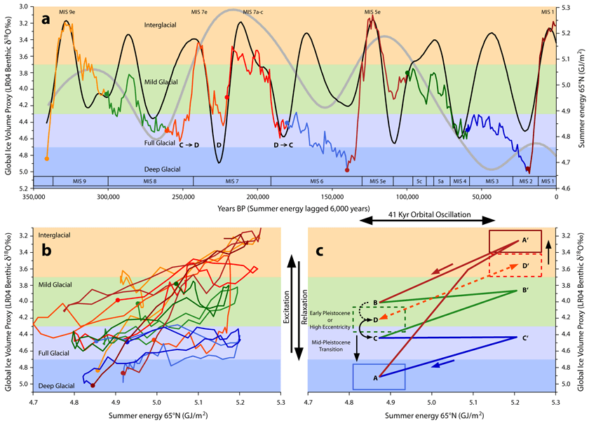
Figure 133 explains how the glacial cycle depends on summer energy (mainly on obliquity), and on ice-volume, and how ice-volume responds to eccentricity. Figure 133a shows an ice-volume proxy (LR04 benthic δ18O) for the past 340 Kyr, overlain by the summer energy parameter that has been lagged by 6000 years, to account for the observed delay of the effect to the forcing (Huybers, 2009; Donders et al., 2018). By plotting ice-volume versus lagged summer energy (figure 133b), it is observed that during the 41-Kyr oscillations in summer energy, ice-volume starts and ends at repeatable states defined following Paillard (1998) as interglacial, mild-glacial, full-glacial, and deep-glacial.
Figure 133. The timing of Pleistocene glaciations as a function of summer energy, ice-volume and eccentricity. a)LR04 benthic stack as an ice proxy (multi-colored line; Lisiecki & Raymo, 2005) for the past 341 Kyr. The line was colored in 40-41 Kyr segments with orange-red tones for low ice segments, green tones for intermediate ice segments and blue tones for high ice segments, and dots of the same color at the start of each segment. Background color defines four different states, light orange for interglacial, light green for mild-glacial, light blue for full-glacial, and cyan for deep-glacial. Black curve is summer energy at 65°N with a 275 W/m2threshold (Huybers, 2006), lagged by 6000 years to compensate the delay between forcing and effect. Thick grey curve is eccentricity (without scale; Laskar, 2004). b)Plot of the multi-colored ice proxy curve versus summer energy. It is evident that the ice volume at the start of the orbital 41 Kyr oscillation in summer energy determines the subsequent ice volume evolution during the oscillation and the possibility of an interglacial taking place in that oscillation. c)Simple excitation/relaxation multi-state model explains the timing of Pleistocene glaciations. Under Early Pleistocene or high eccentricity conditions climate operates as a simple oscillatory system represented by dashed lines, reversibly transitioning at 41 Kyr frequency between mild-glacial (D) and cool interglacial (D’). Mid-Pleistocene transition when eccentricity is not high introduced an ice-volume requirement for excitation out of glacial conditions, represented by the downward arrow (A), and at the same time resulted in warmer interglacials (A’), as the upward arrow indicates. Depending on the speed of ice-volume accumulation, that is inversely correlated to eccentricity, the system must transition through one or two oscillations (two represented, B’ & C’) in the relaxation process to reach the excitable state (A). Low eccentricity favors high ice accumulation accelerating the relaxation (only one oscillation required). Medium eccentricity delays the relaxation as ice accumulates more slowly (two oscillations required). High eccentricity bypasses the ice requirement, returning the system to Early Pleistocene conditions as it happened in the C -> D transition 245 Kyr BP when due to high eccentricity MIS 7e was produced despite low ice-volume and being very late in the summer energy oscillation. The system transitioned back to Mid-Pleistocene conditions after MIS 7a-c (D -> C). The double dependency on ice-volume and eccentricity to produce interglacials results in the absence of a regular pattern. Interglacials are produced at 41, 82, or 123 Kyr intervals. However, the ice-volume dependency on eccentricity results in a 100-Kyr cycle on ice accumulation that is clearly appreciable in ice proxies.
A simple excitation/relaxation model (figure 133c) explains the timing of glaciations. During the Early Pleistocene the situation can be described by a reversible oscillation both in summer energy and ice-volume (dashed bi-directional orange arrow) between mild glacial (D) and cool interglacial (D’) at a 41-Kyr frequency. At the Mid-Pleistocene Transition the cooling of the world caused the beginning of the build-up of extensive continental ice-sheets outside the polar regions during glaciations. Now glacial periods would transition towards more extreme conditions until ice-volume would be so high as to cause high ice-sheet instability (A). This ice-sheet instability is reflected in massive iceberg discharge when perturbed, resulting in Heinrich events. Also, the rebound effect from ice-sheet instability causes warmer interglacials (A’). Mid and Late Pleistocene are characterized by bigger temperature swings between deep glacial and warm interglacial.
When the interglacial ends, the system must relax back to the initial (A) state, but the ice-volume required is so high that it must transition through one or two oscillations (two showed in figure 133c) during which little ice is melted during the summer energy increase (B -> B’, C -> C’), but considerable ice-sheet growth takes place during the summer energy decrease (B’ -> C, C’ -> A). This causes some glacial periods to last one or two complete obliquity oscillations.
Global ice-volume is under control of eccentricity, because high eccentricity enhances the effect of precession and low eccentricity damps it. When eccentricity is very high its effect is like returning to the Early Pleistocene, facilitating an interglacial at every summer energy oscillation. Under very high eccentricity intermediate ice-volume glacials (B, C) behave as Early Pleistocene glacials (D). This can be seen very clearly at the MIS 7e interglacial 245 Kyr ago (figure 133a). As the model indicates, the glacial state prior to MIS 7e was of full-glacial, with an ice-volume insufficient to produce an interglacial, thus little ice was melting despite high summer energy. However, when eccentricity became very high (figure 113a, grey curve), a late interglacial suddenly took place (C -> D transition) with very little time left before low obliquity put an end to it. Then, as eccentricity continued being very high, a new interglacial was produced (MIS 7c-a). Both MIS 7 interglacials happened due to high eccentricity, and they were cool interglacials of the Early Pleistocene type. The effect that high eccentricity has in promoting interglacials and low eccentricity in inhibiting them results in more ice-volume accumulating at times of lower eccentricity. The consequence is that although interglacials do not follow a 100-Kyr eccentricity cycle, ice-volume does present a 100-Kyr cycle (figure 133a).
To study the end of the present interglacial the relevant orbital parameters are summer energy (or obliquity) and eccentricity. By contrast, almost every study dealing with the issue has used the erroneous 65°N summer insolation parameter.
MIS 11c is a poor Holocene analog
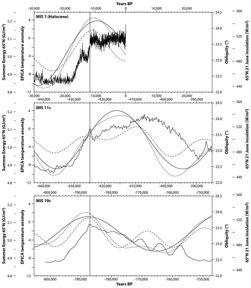
Most authors use MIS 11c interglacial as analog to the Holocene, because of similarly low eccentricity. However, precession and obliquity do not align in the same way for MIS 11c as for the Holocene. MIS 11c is an anomalous interglacial in terms of duration, and clearly this is not due to low eccentricity as MIS 19c had similarly low eccentricity and a standard duration (figure 130).
During the Mid to Late Pleistocene only the combination of high obliquity and high 65°N summer insolation provides enough summer energy to terminate the glacial period. Afterwards (as in MIS 19c, figure 134), the fall in summer energy brings about glacial inception after a delay of several thousand years. In the case of MIS 11c, an unlikely coincidence of several factors working together resulted in the longest interglacial of the past million years. First, 65°N summer insolation was relatively high for many thousands of years before glacial termination, above 480 W/m2(today’s value). This, together with high ice-volume instability, could have “primed” the interglacial, that started unusually soon after summer energy began increasing, without the usual wait to obliquity increase. The obliquity peak took place right in the middle of two insolation peaks. It is extremely unusual that such combination would produce an interglacial in the Mid to Late Pleistocene, but in the case of MIS 11c the 65°N summer insolation at the minimum between the two insolation peaks never falls below 500 W/m2, a value higher than today’s. As a result, summer energy shows a very broad peak of 20,000 years, versus the usual 10-12,000 years. When summer energy was declining, came the second peak in 65°N summer insolation, increasing the temperature and producing a very warm interglacial, particularly so late. When finally, the orbital conditions were adequate for glacial inception the interglacial had lasted almost 25,000 years, almost double the usual duration. The high amount of heat gained during such a long interglacial caused the delay between falling summer energy and glacial inception to be of 10,000 years instead of the usual 6000. MIS 11c ended up lasting close to 35,000 years. However, despite such a long interglacial expanding two precession peaks, it could not extend from one obliquity oscillation to the next. Once glacial inception is reached there is no turning back even under rising obliquity and summer energy.
Figure 134. Low eccentricity interglacials of the past 800 Kyr. EPICA Dome C deuterium proxy expressed as temperature anomaly for MIS 1, MIS 11c, and MIS 19c, aligned at their interglacial start (vertical line). MIS 1 and MIS 19c have a similar orbital configuration with obliquity (continuous line) rising slightly ahead of northern summer insolation (dashed line) producing a peak in summer energy (dotted line) at the start of the interglacial. For MIS 11c northern summer insolation (dashed line), started increasing from a relatively high level several Kyr earlier than obliquity (continuous line), and continued being high for two oscillations resulting in a very wide summer energy peak (dotted line). When obliquity, northern summer insolation, and summer energy decreased for MIS 11c, there was a longer than usual delay until temperature fell. Despite its unusual length due to its unusual orbital configuration, MIS 11c could not continue through an obliquity minimum. The proximity of its obliquity minimum makes the Holocene orbital configuration unfavorable for a long interglacial. Sources: Jouzel et al., 2007; Laskar, 2004; Huybers, 2006.
MIS 19c is a better analog in terms of eccentricity, obliquity, and precession. The main difference is that low values in obliquity and insolation during MIS 19c, and relatively low ice-volume prior to it, resulted in a cool, short interglacial (figure 134). The values of obliquity, insolation, and summer energy were lower at MIS 19c glacial inception than they are currently.
The long interglacial hypothesis
Intermediate complexity (simplified) climate models have been used since the early 1990’s to explore glacial conditions under elevated CO2, and Loutre and Berger (2000) tried to specifically address the question of the end of the present interglacial. They found that at CO2concentrations of 210 ppm the ice-sheets would form at 15 Kyr AP (after present), while no ice-sheets form for 130 Kyr AP with CO2levels of 250 ppm. The 65°N summer insolation changes for the next 50 Kyr are so small that they find that with CO2levels reproducing Eemian Vostok records (a decrease from 296 to 184 ppm over the next 114 Kyr), the present interglacial should last ~ 50,000 years more. Since the only long interglacial of the Mid to Late Pleistocene is MIS 11c, it was confirmed as a suitable analog because it had similarly low 65°N summer insolation changes and relatively high CO2levels (as a warm interglacial).
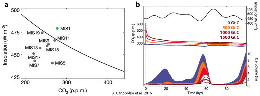
The main conclusions from Loutre and Berger (2000), were that no insolation threshold will be crossed within the next 40 Kyr, and that a glacial inception within the next 50 Kyr would require unnaturally low CO2levels. This modeling result was confirmed multiple times (Cochelin et al., 2006; Mysak, 2008). Archer and Ganopolski (2005) painted a more drastic scenario, with the release of 5000 GtC (545 gigatonnes of carbon were released between 1870-2014) preventing glaciation for the next half million years. Ganopolski et al. (2016) determined a 65°N summer insolation/CO2threshold for glacial inception from model realizations (figure 135a). With such a threshold, not even the pre-industrial CO2level of 280 ppm could produce an interglacial at present (figure 135a), and present cumulative carbon emissions already preclude a glacial inception over the next 50 Kyr (figure 135b).
Figure 135. Model-derived critical insolation-CO2relation and the next glacial inception. a)Best-fit logarithmic relation (black line) between the maximum summer insolation at 65° N and the CO2threshold for glacial inception. The location of previous glacial inceptions in insolation-CO2phase space relative to the best-fit logarithmic curve (grey dots) shows a pre-industrial Holocene (green dot) that could not undergo glacial inception even in the absence of anthropogenic CO2. b)The top panel shows the temporal evolution of the maximum summer insolation at 65° N. The middle panel shows the simulated CO2concentration during the next 100,000 years for different cumulative CO2emission scenarios: 0 GtC anthropogenic emissions (blue), 500 GtC (orange), 1000 GtC (red) and 1500 GtC (dark red line). The bottom panel shows simulated ice volume corresponding to the different CO2emission scenarios. Individual simulations are shown for the 1500 GtC scenario; for the other scenarios, the range is given as shading. Source: Ganopolski et al., 2016.
The long Holocene interglacial hypothesis has become an axiom that is seldom questioned in the scientific literature and fully endorsed by the IPCC. However, this axiom is based exclusively on model studies that rest on three assumptions that have not been demonstrated:
1a. Glacial inception has depended in the past on 65°N summer insolation.
2a. Climate has a high sensitivity to CO2levels. Models produce an average of 3°C/doubling of CO2.
3a. CO2levels remain elevated for tens of thousands of years after a pulse (figure 135b).
If any or all the alternative possibilities were to be correct:
1b. Glacial inception depends on summer energy (obliquity).
2b. Climate has a low to medium sensitivity to CO2, ~ 1.5°C/doubling of CO2.
3b. CO2levels artificially elevated from a pulse can go back down close to baseline over a few centuries.
The prediction would be completely different.
We have already shown evidence that glacial inception is driven by the fall in obliquity, well reflected in summer energy, and not by 65°N summer insolation. Models don’t appear to be as sensitive to obliquity changes as climate. Another thing models ignore is that although low eccentricity promotes small changes in 65°N summer insolation due to a nearly circular orbit, it also clearly promotes ice-volume build up during low summer energy periods. The 100 and 400-Kyr eccentricity cycles are associated with high ice-volume at times of low eccentricity (figure 133a), and present eccentricity is very low and will decrease over the next 25 Kyr. MIS 11c, despite being a very long and very warm interglacial with high CO2levels, was followed by 60 Kyr of small 65°N summer insolation changes, analogous to what awaits in the future. During that period the planet managed to accumulate more ice than during the equivalent period after MIS 5e, when much higher insolation changes and higher eccentricity occurred. Models do not appropriately reflect the 100-Kyr ice cycle paleoclimatologists have recognized for the past five decades.
Not all authors have accepted the unproven model assumptions at face value. Tzedakis et al. (2012) circumvented the problem of CO2sensitivity by trying to determine the natural length of the Holocene under 245 ppm CO2using the MIS 19c analogy. If CO2sensitivity turns out to be low their scenario could be realistic. Their study concludes that with 245 ppm CO2the end of the current interglacial would occur within the next 1500 years.
Vettoretti and Peltier (2004, 2011) have questioned the soundness of the assumption that glacial inception depends on insolation and CO2. They studied separately the effect of the different components of orbital changes, finding that a low obliquity value is most important in determining the strength of the inception process, followed in order of importance by the magnitude of the eccentricity-precession forcing. They also find that areas of perennial snow cover are much more sensitive to the insolation regime than to GHG concentrations. They conclude with a glacial inception at the next obliquity minimum in 10 Kyr in the absence of modern anthropogenic forcing. These results contradict some of the assumptions of the long interglacial hypothesis.
The fat tail of anthropogenic CO2adjustment time
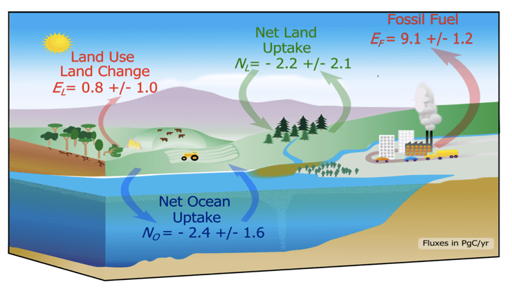
Despite intense research, knowledge of the carbon cycle is still very inadequate. Particularly net carbon fluxes between different reservoirs have a big uncertainty, due in great measure to large differences in regional measurements (Ballantyne et al., 2015; figure 136). Also sink behavior has been a source of significant surprises in the past (Schindler, 1999), due to the unexpected fast growth in net global carbon uptake by ocean and biosphere sinks (Ballantyne et al., 2015). Additionally, models indicate that the fraction of our emissions that remains in the atmosphere (airborne fraction) should increase over time, but we have evidence of the opposite (Keenan et al., 2016). Our imperfect knowledge of the carbon cycle is built into Earth Systems Models (ESM) that from different emissions scenarios produce the atmospheric CO2concentrations that General Circulation Models (GCM, or climate models) use as input. Millar et al. (2017) have shown that the ESMs are working incorrectly, and they contribute to current models running too hot.
Figure 136. Diagram of the global carbon budget. Major fluxes of C to the atmospheric reservoir of CO2 are from fossil fuel emissions (EF) and land use land conversion (EL) and are illustrated as red vectors. Net land (NL) uptake of C from the reservoir of atmospheric CO2is illustrated by green vectors and net ocean uptake (NO) is illustrated by blue vectors. The size of the vectors is proportional to the mass flux of C as indicated in petagrams of C per year. Error estimates for each flux in 2010 are expressed as ±2σ. Error estimates are of the same magnitude as the fluxes. Source: Ballantyne et al., 2015.
Given the problems delimitating and predicting the evolution of the carbon cycle over the past several decades it is surprising that the IPCC would write:
“The removal of all the human-emitted CO2from the atmosphere by natural processes will take a few hundred thousand years (high confidence) … we assessed that about 15 to 40% of CO2 emitted until 2100 will remain in the atmosphere longer than 1000 years” (IPCC AR5 WG1, 2013, page 472).
So, we were unable to predict a few decades ago that over 50% of our fast-growing emissions would disappear from the atmosphere without any time delay, or that the fraction removed could actually increase despite exponentially increasing emissions, yet we have high confidence that 15-40% will remain in the atmosphere 1000 years from now. Clearly, we hugely underestimated the carbon sinks capacity to deal with our emissions, so we cannot have high confidence in distant future predictions. The problem is that we are dealing with a situation without precedent and so the answers that we can obtain from science carry a huge uncertainty that cannot be properly constrained by evidence. The Paleocene-Eocene Thermal Maximum is usually cited as precedent; however, its isotopic carbon excursion took place so long ago that our poor knowledge of its source, amount, and release timescale precludes any meaningful estimation of its decay.
IPCC confidence comes essentially from David Archer’s studies, that since 1997 have become the authority of reference. It is clear that the unburial and release of huge carbon fossil stores constitutes a long-term perturbation of the carbon cycle. Since carbon only permanently exits the carbon cycle very slowly through calcium carbonate sea-bottom burial, and silicate rock weathering, the different compartments of the carbon cycle will have to deal with excess carbon for a very long time and this should necessarily lead to an equilibration between compartments at higher levels than prior to the perturbation. At present the complexity of the effects involved is being studied with box-modeling, but every step in the process requires taking assumptions. It is assumed that the land biosphere, that is currently a sink due to an increase in photosynthesis over respiration, should reach equilibrium within decades after the end of anthropogenic emissions and then become a net source as atmospheric levels decrease. The reduction in atmospheric CO2is then assumed to occur mainly through ocean uptake on a timescale of centuries, driven by changes in oceanic chemistry and ocean mixing. It is assumed that as more carbon dioxide dissolves in the ocean, it will compromise the ocean’s buffering capacity and that ocean acidification will increase the Revelle factor (dissolved CO2to dissolved inorganic carbon). This is then expected to reduce the efficiency of the ocean carbon sink until it stops taking CO2after ~ 1000 years when 14-30% of the maximum level reached remains in the atmosphere (Archer et al., 2005). Higher temperature is also expected to contribute to a decrease in the ocean carbon sink efficiency.
Archer’s (2005) worst case scenario involves anthropogenic emissions of 1600 GtC by 2100 (545 GtC emitted 1870-2014) and increasing afterwards. Up to 1000 GtC should be contributed by a reversal of the land biosphere and soils sinks, and the rest to 5000 GtC total contributed by permafrost and marine methane clathrate deposits. A more realistic scenario considering fossil fuel supply-side constrains and extrapolating observed warming leads to only 500-1000 GtC addition at most. But this amount disregards any effort to reduce emissions, while a higher certainty on CO2climatic effects should lead to more intense efforts to curtail emissions.
It is impossible to have a high confidence that 14-30% of the carbon emitted will remain in the atmosphere 1000 years from now. That number comes from a set of assumptions made using a poor understanding of the carbon cycle, and it could be much lower. Those models are unable to reproduce or explain the significant increase of 20 ppm in CO2that took place between 6000 and 600 BP. Initializing the models at 6000 BP doesn’t produce the pre-industrial CO2levels of 280 ppm, unless ad hocassumptions are introduced, indicating models cannot be trusted to project atmospheric CO2levels thousands of years into the future.
The National Research Council set in 2008 the “Committee on the Importance of Deep-Time Geologic Records for Understanding Climate Change.” This body produced in 2011 the report: “Understanding Earth’s Deep Past: Lessons for Our Climate Future.” This expert committee fully acknowledges the uncertainty present in CO2adjustment time estimates from box-models:
“Although box-model calculations should not be considered definitive, they do suggest that the fossil-fuel perturbation may interfere with the natural glacial-interglacial oscillation driven by predictable changes in Earth’s orbit, perhaps forestalling the onset of the next Northern Hemisphere ‘ice age’ by tens of thousands of years. A more convincing exposition of the central question of “how long” requires more comprehensive models. Scientific confidence in those models will only be high if they can be evaluated against observation. The historical record, and even the expanse of the Quaternary climate record, contains nothing comparable.”
The proposed fat-tail of anthropogenic CO2adjustment time should be taken as a possible scenario if certain assumptions are correct, and not what is expected to happen.
Glacial inception in the Holocene
Glacial inception is the transition from interglacial climate to glaciation, characterized by ice-sheet build up and falling sea-levels. However, there is no unambiguous definition of glacial inception that allows it to be placed at a specific point in time for each interglacial.
In the excitation/relaxation dynamic model of glaciations discussed above (figures 131 & 133), glacial inception can be understood as an irreversible commitment from a quasi-stable interglacial state into a relaxation process towards a stable glacial state, taking place once the conditions that made the interglacial possible have disappeared, and once the downward drift in temperature allows the boundary crossing at the commitment point (figure 131, unstable point).
A point of inflection can be observed in the Antarctic proxy temperature record of past interglacials. In each case the slowly declining temperature of the late interglacial suddenly accelerates into a terminal decline towards glacial conditions (figure 137). In the case of the Eemian interglacial, this inflection point takes place at 120 Kyr BP, when glacial inception has been defined by different criteria (figure 132). It can be shown that the inflection point in the cooling rate corresponds to glacial inception in all cases and can be explained as a point when the intensification of positive feedbacks (like ice-albedo, vegetation changes, or changes in oceanic currents), lead to a steepening of the equator-to-pole temperature gradient and the consequent accelerated cooling of the planet into glaciation.
Figure 137. Interglacial length normalization. The start of an interglacial is defined, as in the Holocene, by the time EPICA Dome C temperature anomaly reaches 0°C, or by extrapolating the rate of warming to the 0°C value. The end of an interglacial is defined at the inflection point where EPICA Dome C temperature anomaly increases its rate of cooling towards glacial values.
The start of an interglacial is also lacking a formal definition. In the case of the Holocene the start is formally placed ~ 11,700 years ago (Walker et al., 2009). At that time EPICA Dome C deuterium proxy temperature record shows no anomaly with respect to current value (0°C anomaly). For a consistent comparison we can define the start of every interglacial at the time they first reach 0°C anomaly in the EPICA Dome C record. For cooler interglacials that didn’t reach 0°C anomaly, picking a lower temperature would lead to overestimating their length, as a lower temperature is reached earlier. A more correct choice is to extrapolate the warming trend to the point where it would have reached 0°C anomaly, picking that time as the normalized start of the interglacial (figure 137; table 3). MIS 13a cannot be normalized and it is not analyzed under the criteria chosen here.
Table 3. Normalized interglacial length. Dates in years BP for the start, end, and length, of normalized interglacials. Dates between parenthesis are extrapolated from the rate of warming. These dates and lengths are used to compare interglacial orbital conditions in the rest of the article.
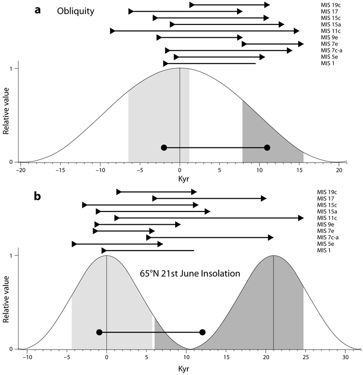
Normalized in this way interglacials are between 10 and 16 Kyr in length, with an average of 13 Kyr, with two exceptions: MIS 7e and MIS 11c. Orbital configuration explains MIS 7e and MIS 11c anomalous length (figure 138). A consistent rule is that all interglacials end when obliquity is low. No interglacial of the past 800 Kyr has gone beyond 15.5 Kyr from the obliquity maximum (figure 138a). Since MIS 7e had a late start with respect to the obliquity cycle it became a very short interglacial. Since MIS 11c started early in the obliquity cycle due to its unusual precessional insolation, it became a very long interglacial. Low eccentricity allows long interglacials when other conditions are present, but it does not cause them to be long.
Figure 138. Interglacial orbital configuration. a)Interglacial start and end dates (triangles) relative to the obliquity maximum. Light grey area indicates interglacial start for all interglacials except MIS 7e and MIS 11c that had an anomalous length due to starting too late and too early respectively in the obliquity cycle. Dark grey area indicates interglacial end for all interglacials. Circles indicate start and end of a typical interglacial with average 13 Kyr length. Interglacials start when obliquity is high and end when obliquity is low. b)Interglacial start and end dates (triangles) relative to the northern summer insolation maximum. Light grey area indicates interglacial start for all interglacials. Dark grey area indicates interglacial end for all interglacials. Circles indicate start and end of a typical interglacial with average 13 Kyr length. Interglacials start when insolation is high but can end at any time in the insolation cycle.
The other orbital rule is that interglacials of the past 800 Kyr start when the combination of obliquity and precessional insolation is high enough (high summer energy). Precessional insolation is irrelevant for glacial inception, as three interglacials were capable of surviving through an insolation minimum, yet they ended close to the next maximum, when obliquity dropped. A typical interglacial (figure 138, line between circles) starts 2000 years before obliquity maximum, and 1000 years before insolation maximum, and lasts 13,000 years. So far, the Holocene is extraordinarily close to a typical interglacial in astronomical terms and length.
Orbital configuration alone can explain when interglacials start and end, while changes in CO2levels cannot. Interglacial temperature is inversely correlated to ice volume (figure 133a; warmer interglacials correspond to previous higher ice-volume), and directly correlated to CO2(figure 110a). And ice-volume is inversely correlated to eccentricity (figure 133a). As it is difficult to explain why CO2levels would inversely correlate to prior ice-volume, the most likely explanation is that CO2levels are a consequence of temperature levels, not a cause (eccentricity -> ice-volume -> temperature -> CO2). Eemian glacial inception and the next 5000 years of cooling took place under stable 270 ppm CO2levels, indicating that glacial inception is responding to orbital changes, not CO2changes. Despite this evidence IPCC expresses virtual certainty that a new glacial inception is not possible for the next 50 Kyr if CO2levels remain above 300 ppm (IPCC, AR5, 5.8.3, 2013). Ice core measurements indicate CO2levels at past glacial inceptions have always been below 300 ppm, but there is simply no evidence indicating how high CO2levels must be to stop a glacial inception, if that is even possible.
It is widely known that there is a delay between the astronomical signal and the geological evidence of climate change, this delay, in the case of obliquity is ~ 6000 years (Huybers, 2009; Donders et al., 2018). The logical conclusion is that the astronomical threshold for glacial inception is crossed ~ 6000 years before it takes place. This inference is supported by the presence at the end of interglacials of a period of declining temperatures before the inflection point that indicates glacial inception has been reached (figure 137). In the Holocene that period is termed Neoglaciation, and it is also observed between 126-120 Kyr BP in the Eemian (figure 132).
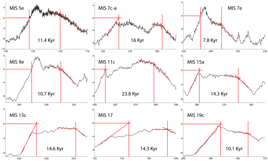
Analysis of the orbital conditions that produce a glacial inception requires examining them 6000 years before the inflection point in the cooling rate at the end of the interglacial. Glacial inception does not take place at 65°N, but at 70°N, where ice sheets start to grow (Birch et al., 2017). Examination of 70°N summer energy (at 250 W/m2threshold) 6000 years before glacial inception (figure 139, diamonds) reveals a threshold at 4.96 GJ/m2when the glacial inception orbital “decision” has already been taken for all previous interglacials. Two interglacials, MIS 9e and MIS 5e, had a much higher summer energy at the orbital decision point. They have in common a well below average duration (10.7 and 11.4 Kyr), probably due to the early decision. They also have in common being warm interglacials at the beginning and suffering a very big drop in Antarctic temperature a few thousand years after starting. This appears to be a feature of short interglacials (figure 137). Whether this early cooling facilitated or caused an early decision to end the interglacial is unknown.
Figure 139. Orbital decision to end an interglacial. Summer energy at 70°N with a 250 W/m2threshold for the past 800 Kyr. Diamonds mark the position 6 Kyr before glacial inception as observed in the EPICA Dome C temperature proxy record for each interglacial except MIS 13. Dashed line marks the lowest value observed (4.96 GJ/m2). Six interglacials were very close to this value 6 Kyr prior to glacial inception. The Holocene (MIS 1) is already below that value.
The 4.96 GJ/m2limit was crossed by the Holocene 1500 years ago, so the orbital decision to end the Holocene has already been taken. By orbital considerations alone the Holocene doesn’t have more than 4500 years left before glacial inception, but it could have as little as 1000 years left if the start of the Neoglaciation 5000 years ago corresponds to the Holocene’s orbital decision. The average duration of Holocene-like interglacials is 13,800 years. That length would place the end of the Holocene, 2000 years from now, right at the center of the obliquity range for the end of every interglacial, 12 Kyr after the obliquity maximum (figure 138a, dark grey area). Between 1500-2500 years from now, there should be a period where two consecutive lows in the Eddy solar cycle separated by a low in the Bray solar cycle are expected, defining a period similar to 8.4-7.1 Kyr BP when eight solar grand minima took place in rapid succession (figure 122). 1500-2500 years from now looks like an excellent time for the next glacial inception.
The analysis of the leading orbital decision to the lagging glacial inception, 6 Kyr later, provides possible answers to some questions, like why the Holocene did not end at the LIA. Since the Neoglaciation started 5 Kyr BP, it is likely that the LIA took place too early, and the interglacial was too young then for glacial inception. The intense cooling accompanied by glacier extension, and a reduction from 280 to 270 ppm CO2(Eemian’s glacial inception level), indicates it was probably a close call, that resulted in a temperature rebound afterwards. Similarly, Ruddiman’s “Early anthropogenic hypothesis” (Ruddiman, 2007), that states that a glaciation was prevented by early agricultural release of greenhouse gases, is unnecessary. With or without human intervention the Holocene should not have ended yet. The question of the GHG increase during the Mid to Late Holocene remains controversial, but it is unrelated to the length of the present interglacial.
The next glaciation
Without human intervention the next glaciation should start in 1500-2500 years. The question that we cannot answer with any degree of certainty is how high CO2levels should have to be to prevent glacial inception. Summer energy is going to be very low for the next 20,000 years and that should require sufficiently elevated CO2levels for that long. Alternatively technology could develop to a point when it is possible for humankind to prevent the next glaciation. Those are questions that cannot be answered, but we can make reasonable inferences from what we do know.
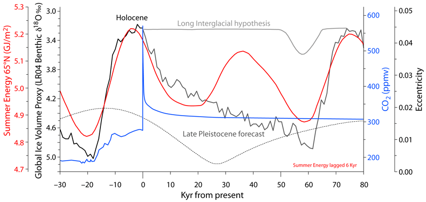
Over the past 150 years it is calculated that we have produced 545 GtC leading to an increase in atmospheric CO2of 125 ppm. Estimates from reputable sources place fossil fuel peak production in a few decades (see 21st Century Climate Change). Even if fossil carbon is more abundant, we might already have extracted one-third to half of what we will extract over the next centuries. Supply constraints should limit our emissions even in the unlikely case that we don’t limit them ourselves as we are already doing. If these estimates are correct, peak atmospheric CO2levels should not go much above 550 ppm (figure 140, blue line). A rapid decline in CO2should follow as oceans and the biosphere absorb most of it, but according to current models about 320 ppm should remain for a very long time (figure 140, blue line; Archer, 2005). If this assumption is correct, the question is if 320 ppm of CO2could stop a glaciation, as the IPCC claims with virtual certainty. We know the Eemian entered glaciation with 270 ppm, 50 ppm below future estimated levels. An opposite result from just 50 ppm difference would require a very high climate sensitivity to CO2. The 93 ppm increase between 1959 and 2018 has been accompanied by climatic variability within interglacial range, as Holocene Climatic Optimum conditions have not been reproduced. Achieving changes of an interglacial-glacial scale might require a much larger amount of GHG than available.
Figure 140. Future climate forecasts for the next 80 Kyr. LR04 benthic stack global ice volume proxy for the past 30 Kyr (black curve; Lisiecki & Raymo, 2005). Orbital eccentricity for the past 30 Kyr and future 80 Kyr (dotted line; Laskar, 2004). Summer energy at 65°N with 275 W/m2threshold for the past 30 Kyr and the future 80 Kyr lagged by 6000 years (red curve; Huybers, 2006). Past CO2levels from ice cores and modeled long term CO2concentration evolution after a 1250 GtC pulse (cyan curve; Archer, 2005). Future global ice volume forecast considering only orbital conditions by reproducing ice volume change after MIS 11c, 402-322 Kyr BP, a period with similar orbital evolution (dark grey curve). Future global ice volume modeled after a 1000 GtC pulse, representing the long interglacial hypothesis (light grey curve; Ganopolski et al., 2016).
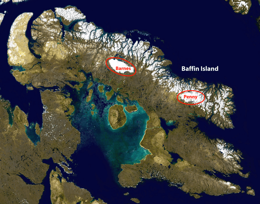
If humankind does not change it, glacial inception should take place in 1500-2500 years. Ice caps at Baffin Island (figure 141) and the Canadian Arctic Archipelago will start to grow, initiating the Laurentide ice sheet (Birch et al., 2017), while ice caps should also grow first over West Siberian islands. Glaciers in Norway should grow to the sea and start releasing icebergs due to increased winter precipitation. The Fennoscandian ice sheet growth, however, should be delayed by an intensification of AMOC, that is expected to bring more heat towards the Nordic seas (Born et al., 2010). In 10,000 years large ice sheets should have developed causing sea level to fall by 30-40 m. Current eccentricity is very low and is going to continue decreasing to almost zero over the next 25 Kyr (figure 140, dotted line). While low eccentricity prevents insolation from going too low, it also prevents it from going too high, so the ice accumulated over low summer energy periods doesn’t melt significantly during periods of higher summer energy. The result is that low eccentricity promotes a faster ice-sheet growth.
Figure 141. Baffin Island ice caps. The Barnes and Penny ice caps in Baffin Island (Canada) are the last remnants of the Laurentide ice sheet of the Wisconsinan glaciation. They are projected to disappear in 300 years if Modern Global Warming continues intensifying (Gilbert et al., 2017). Instead, together with the Canadian Arctic Archipelago and West Siberian islands, they might constitute the starting places for the next glaciation. Source: Public domain from NASA through Wikipedia.
The next high summer energy period in 35 Kyr cannot result in a new interglacial. Obliquity and insolation oscillations are misaligned during that period (not shown), and despite a rapid ice-sheet growth ice-volume should still be too low, so every necessary condition for a Late Pleistocene interglacial is missing in 35 Kyr. Quite the contrary, the low eccentricity should cause the ice-volume to grow through the summer energy peak as it happened during MIS 10 glacial period under similarly low eccentricity (figure 140, dark grey line). On the positive side, the rapid ice-volume accumulation over the next 60 Kyr should create the correct conditions for a new interglacial in 70 Kyr, when a correct orbital alignment and sufficient ice-volume should produce the next interglacial.
If Berger and Loutre (2002), Archer (2005), and Ganopolski et al. (2016) are correct, and the residual CO2in the atmosphere will allow, for the first time in two million years, the survival of an interglacial through an obliquity minimum, then the Holocene should last for at least 50 Kyr more (figure 140, light grey line).
Milankovitch forcing is a very powerful force when acting over millennia. With the help of the appropriate feedbacks it puts the planet into very cold glacial periods and then melts the ice sheets into warm interglacials. It is very difficult for scientists and people in general, living during a multi-centennial warming period characterized by a strong increase in GHG to imagine that on the long run Milankovitch forcing might win. The Romans that for many centuries lived in a warm world characterized by technical progress could not imagine that their mighty empire could fall amid a cooling and worsening climate and terrible plagues into a millennial dark age of lost knowledge and declining civilization. A new glacial period would constitute humankind’s biggest test and clearly has the potential to constitute its worst catastrophe. The precautionary principle requires that we start preparing for that possibility over the next decades and centuries while we are in a warm optimum, as cooling periods are rife with troubles.
For the past 2 million years, when obliquity declined enough a glacial period always followed. Obliquity is declining fast, and we should not have too much confidence on computer models that tell us this time will be different.
Conclusions
1) The glacial cycle fits a model of a stable glacial state that reaches an excitable point where fast excitation (rapid warming) takes it to a quasi-stable interglacial state that slowly degrades to an unstable point where a slow relaxation takes it back to the glacial state. This dynamic system is defined as a fast-slow excitable system around a two-branch slow manifold.
2) Interglacials of the Early Pleistocene, or later when eccentricity is very high, are determined exclusively by summer energy, the amount of energy above a melting threshold accumulated over the entire summer, a parameter that depends mainly on obliquity at high latitudes.
3) After the Mid-Pleistocene Transition when eccentricity is not very high, interglacials are determined by a combination of high summer energy and high ice-volume.
4) This dual interglacial determination that depends on summer energy, eccentricity, and ice-volume, results in an irregular pattern of interglacials after the Mid-Pleistocene Transition, but the negative correlation between eccentricity and ice volume results in a 100-Kyr cycle in ice-volume.
5) Due to the ~ 6000-yr lag between orbital forcing and ice-volume effect, the orbital threshold for glacial inception is crossed ~ 6000-yr before glacial inception. Analysis of the past 800 Kyr indicates the orbital threshold to terminate the Holocene was crossed long ago.
6) In the absence of sufficient anthropogenic forcing, glacial inception might take place in 1500-2500 years as determined by orbital parameters, average interglacial length, Neoglaciation length, and solar variability periodicities.
7) The long interglacial hypothesis rests on the wrong astronomical parameter, high equilibrium climate sensitivity to CO2, and uncertain model predictions of very long-term CO2decay rates. The virtual certainty by the IPCC that a glaciation is not possible for the next 50 Kyr if CO2levels remain above 300 ppm is unsupported by evidence.
Acknowledgements
I thank Andy May for reading the manuscript and improving its English, for his comments and continued support.
Bibliography
JC note: This is the final installment in Javier’s series Nature Unbound. This is a truly remarkable collection of essays, which has provided many insights. A very special thank you to Javier for providing these articles.