A guest post by Nic Lewis
Introduction
Global surface temperature (GMST) changes and trends derived from the standard GISTEMP[1] record over its full 1880-2016 length exceed those per the HadCRUT4.5 and NOAA4.0.1 records, by 4% and 7% respectively. Part of these differences will be due to use of different land and (in the case of HadCRUT4.5) ocean sea-surface temperature (SST) data, and part to methodological differences.
GISTEMP and NOAA4.0.1 both use data from the ERSSTv4 infilled SST dataset, while HadCRUT4.5 uses data from the non-infilled HadSST3 dataset. Over the full 1880-2016 GISTEMP record, the global-mean trends in the two SST datasets were almost the same: 0.56 °C/century for ERSSTv4 and 0.57 °C /century for HadSST3. And although HadCRUT4v5 depends (via its use of the CRUTEM4 record) on a different set of land station records from GISTEMP and NOAA4.0.1 (both of which use GHCNv3.3 data), there is a great commonality in the underlying set of stations used.
Accordingly, it seems likely that differences in methodology may largely account for the slightly faster 1880-2016 warming in GISTEMP. Although the excess warming in GISTEMP is not large, I was curious to find out in more detail about the methods it uses and their effects. The primary paper describing the original (land station only based) GISTEMP methodology is Hansen et al. 1987.[2] Ocean temperature data was added in 1996.[3] Hansen et al. 2010[4] provides an update and sets out changes in the methods.
Steve has written a number of good posts about GISTEMP in the past, locatable using the Search box. Some are not relevant to the current version of GISTEMP, but Steve’s post showing how to read GISTEMP binary SBBX files in R (using a function written by contributor Nicholas) is still applicable, as is a later post covering related other R functions that he had written. All the function scripts are available here.
How GISTEMP is constructed
Rather than using a regularly spaces grid, GISTEMP divides the Earth’s surface into 8 latitude zones, separated at 0°, 23.58°, 44.43° and 64.16° (from now on rounded to the nearest degree). Moving from pole to pole, the zones have area weights of 10%, 20%, 30%, 40%, 40%, 30%, 20% and 10%, and are divided longitudinally into respectively 4, 8, 12 16, 16, 12, 8 and 4 equal sized boxes. This partitioning results in 80 equal area boxes. Each box is then divided into 100 subboxes, with equal longitudinal extent, but graduated latitudinal extent so that they all have equal areas. Figure 1, reproduced from Hansen et al. 1987, shows the box layout. Box numbers are shown in their lower right-hand corners; the dates and other numbers have been superseded.
Figure 1. 80 equal area box regions used by GISTEMP. From Hansen et al. 1987, Fig.2.
Where the distance from a land meteorological station to a subbox centre is less than a gridding radius (limit of influence), normally set at 1200 km, its temperature anomalies[5] are allowed to influence those of that subbox.[6] Figure 3, reproduced from Hansen et al. 1987, illustrates the areas thereby influenced in 1930 by the set of stations originally used. Almost all land outside Antarctica was by then within 1200 km of a meteorological station. Coverage was slightly poorer in 1900.
The 1200 km limit of influence was set to equal that at which the average correlation of annual temperature changes between pairs of stations falls to 0.5 at mid and high latitudes, or 0.33 at low latitudes. It is implicitly assumed that correlation of annual changes is indicative of similarity of trends, which may not be entirely accurate. Hansen et al. 1987 found no directional dependence of annual correlations, but while temperature trends have no general longitudinal dependence they do vary systematically by latitude.
Figure 2. Distribution of land stations and their 1200 km radii of influence in 1930. From Hansen et al. 1987, Fig.1.
Subboxes in ice free ocean areas use SST data – and are therefore not subject to influence by land stations within the 1200 km limit – whenever it is available, provided that at least 240 months SST data exist and that at no time was there a land station within 100 km of the subbox centre.[7] Although ERSSTv4 SST data is complete in ocean areas, Hansen et al. 2010 stated that SST data is only used in regions that are ice free all year. The effective ocean area is on this basis reduced by 10%, to 64% of the global surface area, from its actual fraction of 71%. Although the Hansen et al. 2010 statement seems to be inaccurate,[8] in most calendar months SST data appears to be used only over a fairly small fraction of the ocean north of 60°N and south of 60°S.
Figure 3, reproduced from Hansen et al. 2010, shows the ice-free ocean area. The added lines showing the extent of the GISTEMP polar latitude zones. Their position indicates that temperature anomalies in those zones are dominated by land station data. The use of land station data to infill temperatures over sea ice hundreds of kilometres away appears to provide a preferable measure of surface air temperature to the use of equally distant SST data (or to setting the temperature in sea ice cells to seawater freezing point), provided the intervening sea ice cover is almost complete. Where, however, a significant proportion of the ocean surface in or near the grid cell concerned is open water, as in areas of broken sea ice, it is not clear that using land temperatures is appropriate.
Figure 3. Ice-free ocean area in which GISTEMP uses SST data. From Hansen et al. 2010 Fig. A3, with
lines (red) added showing boundaries of the northern and southern polar boxes latitude zones.
Records for each box are built up by combining records from each constituent subbox with data, equal-weighted, after first converting them to anomalies.[9] Records for each latitude zone are then built up from each constituent box, weighted according to the number of its subboxes with data.
A peculiarity of the GISTEMP method for combining land and ocean data is that their relative weight in each latitude zone, and hence the global, temperature anomaly time series changes over the record, as the availability of land station data varies. It also depends on the limit set for a land station’s influence. With a 1200 km limit variation in the relative land and ocean weights should be small after 1900 save in the southern polar latitude zone, but with a smaller limit the variation would be larger and the land weight might increase significantly over time. Prior to 1900 the land weighting may have been materially too low in the two tropical latitude zones, at least, even with a 1200 km limit.[10]
The GISTEMP global record was originally created by combining latitude zone temperature anomalies weighted in the same way. But in 2010 an important change was made. In subsequent versions of GISTEMP, latitude zone anomalies have been weighted by each zone’s area, even if it only has defined temperature changes over part of its area.
The relevance of the 1200 km limit of influence
Hansen et al. 1987 stated that using alternatives to the 1200 km limit on a station’s influence had no significant effect on global temperature changes. Hansen et al. 2010 stated more specifically that the global mean temperature anomaly was insensitive to the limit chosen for the range from 250 to 2000 km, and that the GISS Web page provides results for 250 km as well as 1200 km. In support of this insensitivity, it gave the 1900–2009 linear trend based change in global mean temperature as 0.70°C with a 1200 km limit and 0.67°C with a 250 km limit.
I was surprised that the GMST trend was not more affected by the limit on a station’s influence, and decided to examine the sensitivity for the current GISTEMP version. Unfortunately, GISS appears no longer to provide global mean LOTI data using a 250 km limit on their Web pages. However, very commendably, GISS makes available computer code to generate GISTEMP.[11] The code has recently been rewritten in the modern language Python and, although I am unfamiliar with that language, the code and procedure for running it are well documented and I found it simple to run and to modify parameters it uses.[12]
I checked my results, with the gridding radius set at the standard 1200 km, against those from output on the GISTEMP web pages.[13] The global trends were within 0.01°C/century of each other over 1880-2016, 1900-2009 and 1979-2016. The linear trend based change in GMST over 1900-2009 I obtained was 0.89°C, a remarkable 27% higher than that given in Hansen et al. 2010.
Global mean comparisons
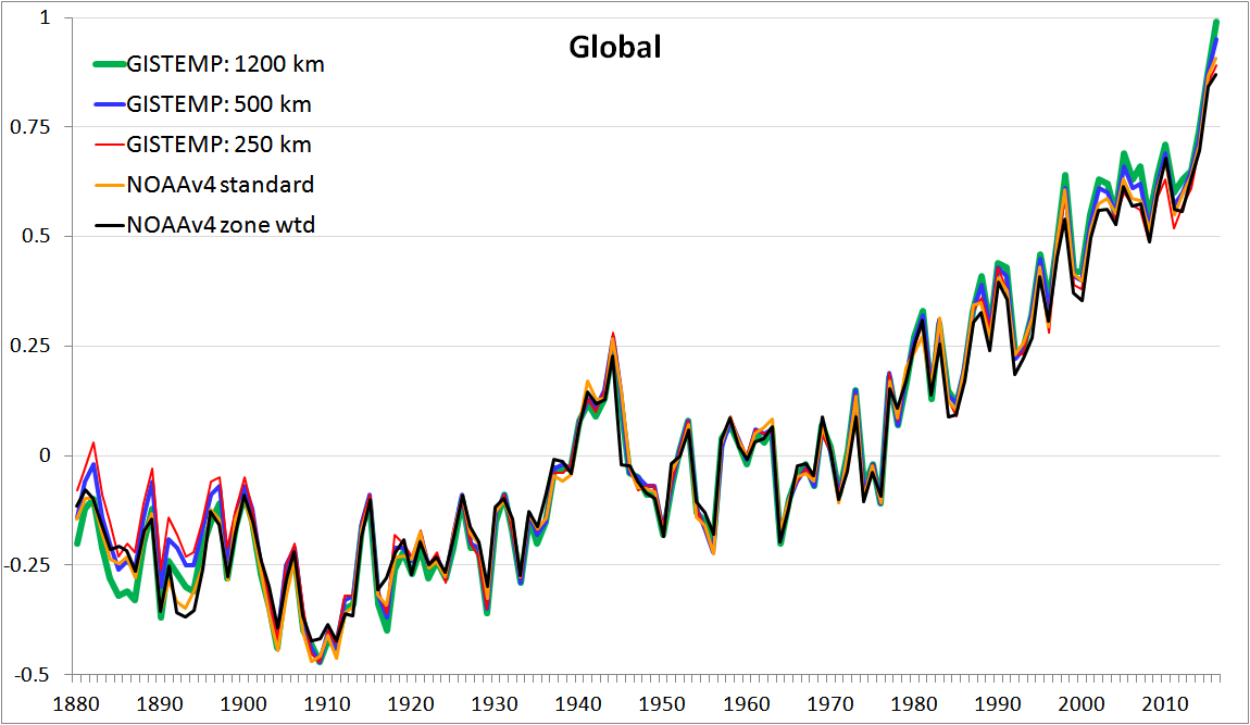
Figure 4 shows a plot of global temperature computed for GISTEMP using 1200 km (green) and 250 km (red) limits on land stations’ influence, and also on an intermediate 500 km limit (blue). It is relevant to show the NOAAv4 global time series (orange) for comparison, as like GISTEMP it is based on ERSSTv4 ocean and GHCNv3.3 land data.[14] Unlike the post-2010 version of GISTEMP, NOAAv4 area weights the temperature anomalies of all cells with data.[15] To provide a fairer comparison with GISTEMP, I have computed a NOAAv4 global time series (black) giving, as for post-2010 GISTEMP, a full area weight to each of the eight GISTEMP zonal latitude bands irrespective of how many of the cells in it have data.[16]
.
Figure 4. Global temperature anomalies (°C) for GISTEMP at different limits of influence, and for
NOAAv4.0.1 area weighted by grid cells with data (standard) or by 5° latitude bands with data
Although all the global time series follow each other closely over most of the record, there are clear differences in the first half century or so and over the last few decades. In the late 1800s, and to a modest extent during most of the 1915-1935 period, the GISTEMP 1200 km line tends to lie below the other lines, although the NOAA lines fall some way below it for several years in the 1890s. Contrariwise, in the late 1800s the GISTEMP 250 km line generally lies above the other lines, with the GISTEMP 500 km line next. Over the last few decades, the GISTEMP 1200 km line is generally the highest, followed by the GISSTEMP 500 km line. These tendencies are reflected in the linear trends for the different global time series over various periods, given in Table 1.
Dataset / trend period
1880-2016
1880-1950
1950-2016
1979-2016
GISTEMP 1200 km
0.72
0.37
1.42
1.72
GISTEMP 500 km
0.66
0.28
1.38
1.64
GISTEMP 250 km
0.62
0.22
1.30
1.52
NOAAv4 standard
0.68
0.37
1.35
1.62
NOAAv4 zone weighted
0.65
0.34
1.29
1.60
Table 1. Linear trends in GMST (°C/century) by dataset and period
The GISTEMP GMST trend I obtain over the full 1880-2016 record is 0.72°C/century when using a 1200 km gridding radius. When this limit of influence is reduced to 250 km, the trend becomes 0.62°C/century. So, using a 1200 km limit rather than 250 km now leads to a 16% higher full record trend, rather than the 4½% higher trend as reported in Hansen et al. 2010. Slightly over half the difference appears to relate to the early decades of the record. The average GMST anomaly over 1880-1900 was approaching 0.1°C warmer when a 250 km rather than 1200 km limit of influence was used. However, a substantial part of it arises over recent decades, when global land station coverage is much more complete. Over 1979-2016 the GMST trend is 1.72°C/century with a 1200 km limit of influence, but only 1.52°C/century with a 250 km limit. So, the claim in Hansen et al. 2010, the latest paper documenting GISTEMP, that the global mean temperature anomaly – and by implication the trend in GMST – is insensitive to the limit on a station’s influence over the range 250 km to greater than 1200 km is simply not true in relation to the current version of GISTEMP.
Examining temperature anomaly time series for the latitude zones where varying the limits of influence has the greatest effect provides some insight into the sources of the trend differences. It turns out that the largest contributions to differences in the 1880-2016 GMST trend come from the polar zones.
Southern polar zone comparisons
Figure 5 shows time series for the 90S-64S GISTEMP latitude zone at different limits of influence.
.
Figure 5. 90S-64S latitude zone temperature anomalies (°C) at different limits of influence (km)
The 90S-64S latitude zone time series at 1200 km influence limit is remarkable. The wild swings between 1903 and 1943, not exhibited to any extent when a limit is set at 250 km or 500 km, turn out to be caused by a single meteorological station, Base Orcadas, located in the South Orkney islands, some way outside this latitude band. The South Orkney Islands have a climate of transition to polar cold weather, not participating in the polar regime; weather conditions can vary markedly from year to year.[17] Despite it being at 60.7°S, the centres of 18 subboxes in the 90S-64S zone are within 1200 km of Base Orcadas. Although a station’s weight in a subbox declines linearly with distance of the subbox centre from the station, reaching zero at its limit of influence, in the absence of other data for the subbox the station’s influence does not diminish until the limit is reached.[18] As there were no other data for the 18 subboxes involved, their temperature anomalies were set equal to those of Base Orcadas. And because there were very few observations in this latitude zone until after WW2 – a smattering of ship SST readings in the ice-free ocean area during summer months – the Base Orcadas data dominated the southern polar zone temperature anomaly for the 1200 km limit time series over 1903-1943; its weight only fell below 33% in 1955.[19]
After working this out, I found that the influence of Base Orcadas on GISTEMP’s 90S-64S zone had been pointed out back in 2009.[20] However, at that time the effect on GISTEMP’s global time series was completely negligible, as until 2010 the weight given to each latitude zone in determining the GMST anomaly was proportional to the area in it for which there was data, which for the 90S-64S zone was only a small fraction of its total area prior to 1955. However, in 2010 GISTEMP switched to weighting each latitude zone by its full area irrespective of how many of its subboxes had data.
Are changes in temperature at Base Orcadas representative of those for the 90S-64S zone, which is dominated by continental Antarctica and the ocean adjacent to it? I very much doubt it. For a start, the correlations of annual temperature changes at Base Orcadas with those at stations in the interior of Antarctica (with records starting circa 1957) are low.
With Base Orcadas dominating them, temperature anomalies for the 90S-64S zone during the first decade or so after 1903 and during the 1930s were generally strongly negative. By contrast, those from data restricted by a 500 km or 250 km limit of influence were only weakly negative, which mirrors much more closely the behaviour of anomalies in the adjacent 64S-44S zone, where data was much less sparse. In my view, the standard GISTEMP methodology is unsuitable for application in the southern polar zone prior to the mid 1950s. While the influence of Base Orcadas on GMST trends is only minor, it is not completely negligible even over the entire record. If pre-1955 Base Orcadas data is removed, the GISTEMP 1880-2016 GMST trend, with a 1200 km limit of influence, falls by 0.01°C/century – over a quarter of the excess of the GISTEMP trend over that for the standard version of NOAAv4.
One other unusual feature of GISTEMP in this latitude zone is that it uses a reconstructed record for Byrd station in Antarctica, the only location in the interior of West Antarctica with a useful pre-1981 record. The reconstruction stitches together, without any offset, the records of two stations having somewhat different locations, construction and instrumentation, and whose records are separated by some years. This procedure, which produces a fast warming record for Byrd, is not in accordance with normal practice for temperature datasets. The reconstructed Byrd record is not used by in HadCRUT4v5 nor to my knowledge in any other dataset apart from the Cowtan & Way infilled version of HadCRUT4. However, its contribution to the GISTEMP global temperature trend is very small.[21]
Linear trends for the different 90S-64S time series over various periods are given in Table 2.
Dataset / trend period
1880-2016
1880-1950
1950-2016
1979-2016
GISTEMP 1200 km
0.60
-1.54
1.25
0.71
Ditto ex Orcadas pre 1955
0.27
-1.30
1.32
0.70
GISTEMP 500 km
0.23
-1.10
1.06
0.56
GISTEMP 250 km
0.10
-0.75
0.72
0.94
NOAAv4 zone weighted
0.08
-0.66
0.35
-0.86
Table 2. Linear trends in 90S-64S anomalies (°C/century) by datasets and period
The GISTEMP 1200 km limit southern polar temperature trend over the satellite period, 1979-2016, during which Base Orcadas had limited influence, exceeded that using a 500 km limit.[22] A comparison with ERAinterim, arguably the best reanalysis dataset, suggests that the standard GISTEMP 1200 km limit version produced an excessive trend in southern polar latitudes since 1979.[23]
Northern polar zone comparisons
I now turn to GISTEMP’s northern polar zone. Figure 6 shows time series for the 64N-90N GISTEMP latitude zone. Here, there are noticeable differences between the various datasets in both early and late decades in the record. These differences are larger than for the southern polar zone, if one ignores the impact of Base Orcadas, despite data being less sparse in the northern than the southern polar zone, especially early in the record.
Figure 6. 64N-90N latitude zone temperature anomalies (°C) at different limits of influence (km)
The lower temperature anomalies up to 1900, relative to those over the stable period from 1903 to 1916, when using the 1200 km limit of influence are questionable. The NOAAv4 dataset weighted in the same way as GISTEMP shows a considerably smaller increase, as (to a lesser extent) do the 250 km and 500 km limit GISTEMP versions. The Cowtan & Way infilled version of HadCRUT4.5 warms only a third as much as the standard 1200 km GISTEMP version in this latitude zone between these two periods.
Linear trends for the different 64N-90N time series over various periods are given in Table 3.
Dataset / trend period
1880-2016
1880-1950
1950-2016
1979-2016
GISTEMP 1200 km
1.77
2.85
3.16
5.74
GISTEMP 500 km
1.60
2.61
3.02
5.44
GISTEMP 250 km
1.42
2.32
2.75
4.96
NOAAv4 zone weighted
1.11
1.68
2.39
4.34
Table 3. Linear trends in 64N-90N anomalies (°C/century) by datasets and period
The large divergence between all GISTEMP variants and NOAAv4 in the 64N-90N latitude zone almost certainly relates to the treatment of sea ice. In a non-infilled record like HadCRUT4, cells with sea ice have no data; their temperature anomaly is effectively treated as always equalling the mean for the region over which anomalies are averaged. In HadCRUT4 this is entire hemispheres, although it would be possible instead to average over latitude zones, as in GISTEMP.[24] In NOAAv4, the spatially complete ERSSTv4 ocean data is used in cells with sea ice. The temperature for such cells is set to -1.8°C, near the freezing point of seawater. In GISTEMP, as the ERSST SST data is flagged as missing in subboxes with sea ice, their temperature anomalies are set equal to those of any land stations with data within the 1200 km (or 500 or 250 km) limit of influence, on a distance-weighted basis where more than one such land station exists. The Cowtan & Way infilled version of HadCRUT4 effectively does much the same through its use of kriging.[25]
Insofar as temperatures over sea ice do reflect those of land temperatures within the radius of influence used, the NOAAv4 method can be expected to understate surface air temperature changes for cells with sea ice; this is also so (to a lesser extent) for the HadCRUT4 method.
It is unclear why the 1200 km GISTEMP version has warmed faster than the 250 km and 500 km versions in 64N-90N in recent decades. Possibly it reflects a higher weighting being given to the highest latitude land stations, and an even lower weighting being given to the very small ice free ocean area included in the zone. Comparisons with the ERA reanalysis dataset suggest that the GISTEMP 1200 km limit version produced realistic trends in arctic temperatures from 1979 until the late 2000s, with a slight underestimation of warming since then.23
Conclusions
The answer to the question originally posed, “How dependent are GISTEMP trends on the gridding radius used?”, is that they are much more dependent than claimed, with use of a 250 km, rather than the standard 1200 km, limit producing materially lower GMST trends over all periods investigated. That does not mean use of a 250 km limit produces a more accurate record. In my view, a 1200 km limit is in general preferable to a 250 km limit, although use of some intermediate value between 500 km and 1200 km might be best. In any event, a 1200 km limit is clearly unsuitable for use in the southern polar zone prior to the middle of the 20th century, since doing so results in unrepresentative temperatures at Base Orcadas – some way outside that zone – dominating temperature changes for the entire 90S-64S zone.
In principle, GISTEMP as currently constructed has several features that arguably make it more suitable for comparisons with global climate model simulations of surface air temperature than HadCRUT4 or NOAAv4, the most prominent other global temperature datasets.[26] GISTEMP:
- gives a full area weight to all latitude zones (unlike HadCRUT4)
- uses nearby land temperatures rather than SST to estimate temperatures where there is sea ice
- uses ocean temperature data that were until recently tied, on decadal and longer timescales, to marine air temperature rather than SST records.[27]
However, against this GISTEMP has a few problematic features that seriously detract from its suitability as a global temperature dataset. GISTEMP:
- fails to ensure ice-free ocean temperature anomalies are weighted by the area they represent
- uses a simplistic infilling method that sets cell anomalies equal to the weighted average of those for land stations up to 1200 km away, with no kriging-like reversion towards the mean with distance.
By contrast, the Cowtan & Way infilled version of HadCRUTv4.5 does not suffer from either of these shortcomings, while matching GISTEMP as regards all but one of its positive attributes identified for making comparisons with climate model surface air temperature data. And while HadCRUTv4.5, and hence Cowtan & Way, use HadSST3 for ocean temperatures rather than the marine air temperature data linked ERSSTv4 dataset, over 1880-2016 the two datasets have essentially identical global trends.[28] Although simulations by the vast majority of global climate models show that ocean surface (2 m) air temperature warms marginally faster than SST, it is not clear that their behaviour in this respect correctly reflects reality. Such models do not properly represent the surface boundary layer, within which steep temperature gradients exist; their uppermost ocean layer is typically 10 m deep. The fact that HadSST3 has warmed as fast as ERSSTv4 (and HadNMAT2) suggests that ocean surface air temperature may not actually warm any faster than SST.
If one is after a globally complete dataset for comparison with global climate model simulations, the Cowtan & Way infilled version of HadCRUT4 therefore looks a better choice than GISTEMP. Interestingly, it is only prior to 1890 and during the last decade that the Cowtan & Way GMST estimate systematically differs from the unfilled HadCRUT4v5 one; the two datasets’ 1890-2006 trends differ by under 1%. IMO, no infilling technique will be that successful prior to 1890 – there isn’t enough data to go on, and data accuracy is also an issue. It is much more plausible that HadCRUT4v5 understates warming since the early years of the 21st century, a period when the Arctic – where there are limited in-situ temperature measurements – warmed very fast. However, over the fifteen years to 2016 the HadCRUT4v5 and Cowtan & Way GMST trends, of 0.138°C /century and 0.160°C /century respectively, are equally close to the 0.149°C /century ERAinterim trend; the GISTEMP and NOAAv4.0.1 trends are both above 0.17°C /century.
Nic Lewis
[1] GISTEMP LOTI, combined land and ocean data: see https://data.giss.nasa.gov/gistemp/
[2] Hansen, J.E., and S. Lebedeff, 1987: Global trends of measured surface air temperature. J. Geophys. Res., 92, 13345-13372, doi:10.1029/JD092iD11p13345.
[3] Hansen, J., R. Ruedy, M. Sato, and R. Reynolds, 1996: Global surface air temperature in 1995: Return to pre-Pinatubo level. Geophys. Res. Lett., 23, 1665-1668, doi:10.1029/96GL01040
[4] Hansen, J., R. Ruedy, M. Sato, and K. Lo, 2010: Global surface temperature change. Rev. Geophys., 48, RG4004, doi:10.1029/2010RG000345
[5] Changes from the mean for the corresponding month over a reference period.
[6] Stations without, for at least one month, data for a total of 20 or more years are dropped.
[7] Hansen et al. 1996 states that “A coastal [sub]box uses a meteorological station if one is located within 100 km of the box centre.” But in fact, if there was at any time a station within 100 km GISTEMP throughout the record uses data from all land stations within 1200 km.
[8] It is unclear whether the GISTEMP code accurately implements this condition. The GISS-pre-processed ERSSTv4 data it uses appears to have had subbox SST data removed throughout the record but by individual month rather than for all year. I presume data was removed for all calendar months in which the subbox concerned contained sea ice in any year of the record. If SST data remain for at least two calendar months then the 240 months minimum data requirement will be met and SST data used for those calendar months. The presence of sea ice appears to be deduced from the subbox SST being cooler than –1.77°C. It is not evident that the ice-free condition was applied before 2010, but it was irrelevant when GISTEMP started using ocean SST data since then used dataset only covered 45°S–59°N.
[9] Curiously, monthly means over 1961-1990 are subtracted to compute subbox temperature anomalies, while an anomaly reference period of 1951-1980 is used when combining subboxes into boxes.
[10] Judging from the January 1886 land coverage for HadCRUT4 shown in Figure 5 of Morice CP, Kennedy JJ, Rayner NA, Jones PD, 2012. Quantifying uncertainties in global and regional temperature change using an ensemble of observational estimates: The HadCRUT4 dataset. J. Geophys. Res. 117: D08101..
[11] The data files it uses are GISS supplied, with sea-ice affected areas of ERSSTv4 data already masked out and the reconstructed Byrd record substituted for the original.
[12] The GISTEMP code is available via https://data.giss.nasa.gov/gistemp/sources_v3/. I used frozen data files from the provided input.tar.gz file, both for speed of processing and to ensure consistent results from different runs. The data files were dated 18 January 2017; slightly different results may be obtained if downloaded current data is used instead, as some pre 2017 values may have been revised. I ran the code on a 64 bit Windows 7 computer with the Anaconda36 implementation of Python, which includes required library modules, installed.
[13] File https://data.giss.nasa.gov/gistemp/tabledata_v3/ZonAnn.Ts+dSST.csv, downloaded 4May17. I also checked the trends produced by the Python code against those I calculated from a global time series produced by weighting each month the anomalies for individual boxes making up each latitude zone by the number of subboxes with data to give zonal anomalies and then combining these latitude zone anomalies, area-weighted. They were almost the same globally.
[14] NOAAv4 anomalies, which are relative to the 1971-2000 mean, have been restated relative to the 1951-1980 mean used by GISTEMP.
[15] In NOAA’s case, 5° latitude by 5° longitude grid cells, not equal area subboxes. However, cell anomalies are area weighted when combined to give zonal anomalies, so the difference should in principle be unimportant.
[16] To simplify the calculations, I reduced the monthly grid cell series to annual mean anomalies before rather than after combining them into zonal latitude bands and then a global time series. NOAA grid cells falling into two GISTEMP zonal latitude bands had their area weight split appropriately. As in GISTEMP, zonal anomalies were derived by combining on an area-weighted basis anomalies for all cells in the zone with data, but each zonal anomaly was given a full weight in computing the global anomaly irrespective of for what proportion of its area cell data existed. Note that a similar comparison is not given for other global temperature datasets since they do not use ERSSTv4 data.
[17] Argentina National Meteorological Service http://www.smn.gov.ar/serviciosclimaticos/?mod=elclima&id=68
[18] Since with only one data source the divisor in the calculation of the weighted subbox anomaly is the same as the weight given to that data source.
[19] Between 1945 and the mid-1950s, both 1200 km and 500 km limit 90S-64S zonal anomalies were also influenced by data from Esperanza Base station, located near the tip of the Antarctic peninsula, 1° outside the zone.
[20] https://chiefio.wordpress.com/2009/11/02/ghcn-antarctica-ice-on-the-rocks/#comment-1471
[21] The inclusion of the reconstructed 1957-2016 Byrd record nevertheless increases the 1957-2016 warming trend in GISTEMP’s 90S-64S region by approximately 0.25 °C/century, compared to when using the original Byrd and Byrd AWS records.
[22] Use of a 250 km limit gave the highest trend over the 1979-2016 period, due to it producing lower temperature anomalies in the 1980s and 1990s.
[23] Simmons, AJ et al., 2017. A reassessment of temperature variations and trends from global reanalyses and monthly surface climatological datasets. Q. J. R. Meteorol. Soc. 143: 101–119, DOI:10.1002/qj.2949. The comparison is for the a 30 degree latitude band around the pole.
[24] I did this in 2014 using 10° latitude zones; the effect on HadCRUT4 GMST trends was very small (zero over 1850-2013), indicating that sparse polar coverage in HadCRUT4 has not of itself led to any significant bias in GMST estimation.
[25] Although as the distance away from any station falls the anomaly for a cell with sea ice will gradually tend towards the global mean land anomaly.
[26] A potential understatement of warming arising from use of temperature anomalies when sea ice cover reduces has however been pointed out (Cowtan, K., et al., 2015: Robust comparison of climate models with observations using blended land air and ocean sea surface temperatures, Geophys. Res. Lett., 42, 6526–6534). This occurs even when sea ice anomaly temperatures are land-based, as the change to SST in temperature anomaly terms is generally less than the change in absolute temperature. However, bias arising from using temperature anomalies when sea ice cover is reducing is likely to be substantially smaller than suggested by the climate model simulations carried out by Cowtan et al., since the reduction in Antarctic sea ice extent simulated by climate models during the period over which they find a bias developing has not occurred in the real world.
[27] In ERSSTv4 ship sea surface temp (SST) measurements, on decadal and longer timescales, are adjusted to match movements in night-time marine air temperature data (per the HadNMAT2 dataset).
[28] As they do over the ice-free 60S-60N latitude zone, which is more relevant to their use by GISTEMP and Cowtan & Way.