by Donald Rapp
On the terminations of Ice Ages.
Terminations occur on solar up-lobes
There is no doubt that there is merit in the widely accepted Milankovitch theory that Ice Ages and their terminations are controlled by solar input to the NH in mid-summer. It is also clear that relying on the solar input to the NH alone, does not adequately account for the occurrence of terminations of Ice Ages. The variation of solar input to high latitudes is modulated by precession, which produces continual up-lobes and down-lobes in solar input with a ~ 22,000-year period. While every termination is accompanied by the 5,500-year rising portion of an up-lobe in the solar input to high latitudes, many strong up-lobes do not produce a termination.
Many solar up-lobes do not produce terminations
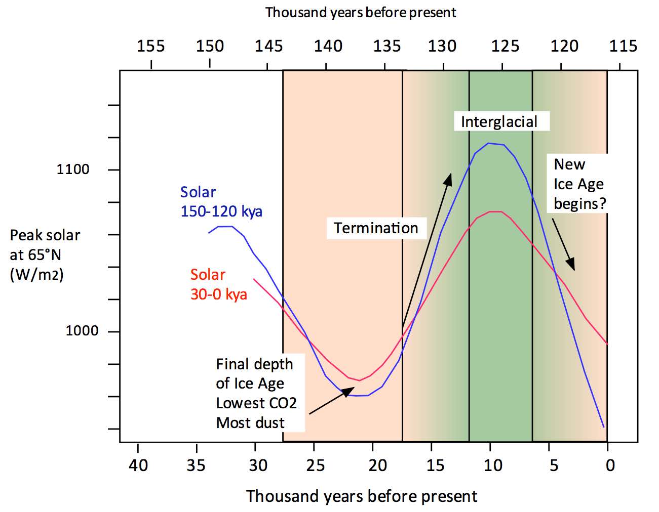
While essentially all terminations occur soon after a significant increase in solar intensity, there are many such increases in solar intensity that do not produce terminations, and the termination around 400 kya is not explainable at all by this argument. Figure 1 shows the relative peak summer solar intensity at 65°N vs. year, along with the occurrences of the various terminations. We may regard the pattern of variability of peak solar intensity in Figure 1as a rapidly varying (~22,000-year period) contribution due to precession of the equinoxes, with an envelope whose amplitude depends on the more slowly varying obliquity and eccentricity. In a sense, this is like an amplitude-modulated radio wave where a high-power “carrier wave” is modulated in amplitude by the signal (in our case eccentricity and obliquity). The key fact is:
There are many sharp up-lobes, but only a fraction of them are associated with terminations. Hence, a sharp up-lobe in solar intensity might be necessary for a termination, but it is certainly not sufficient.
Figure 1. Solar input to 65°N at midsummer shown along with the termination ramps from Rothlisberger et al.(2008).
Need for an X-factor to accompany solar up-lobes at termination
At least one other factor must be compounded into the overall model for why and when terminations occur. After reading many dozens of learned papers on terminations of Ice Ages, I have come to the tentative conclusion that over the past 800,000 years, the natural state of the Earth was that of what we call an “Ice Age”. Apparently, Ice Ages occurred because the energy balance of the Earth in pre-industrial times favored production of ice sheets in the North, and the ice sheets were enhanced when the solar input to the NH was unusually low. Even during periods with rising lobes in the pattern of solar input to the NH, Ice Ages persisted in the absence of another factor(s) that forced origination of a termination. After a termination, an Interglacial ensued. Apparently, this “X-factor(s)” diminished and eventually disappeared during an Interglacial. When the X-factor(s) was no longer operating, the gradual growth of ice sheets resumed from their depleted condition after a termination. The new Ice Age took many tens of thousands of years to mature, but ultimately, a new global maximum of the ice sheets was reached.
So, what we had was not, as one might tend to perhaps assume, unusual Ice Ages that interfered with natural periods of relative warmth. Instead, we had persistent Ice Ages that were intermittently terminated when the X-factor(s) arose, as an exception to the rule, rather than as a state of normalcy. The terminations were the exceptions.
Therefore, the search for the holy grail of Ice Ages is essentially the search for the X-factor(s) that causes terminations, along with rising solar input to the NH.
It is interesting that Wolff et al.(2016)understood the need for the X-factor(s). They said:
Milanković theory would suggest that terminations (and associated interglacial onset) should occur on the rising limb of NH summer insolation. As not every precessional cycle leads to an interglacial, there must be another factor that leads to Interglacials occurring in some precessional cycles and not others.
The “doom” blog (one of the more credible climate discussion blogs),[1]reviewed many theories and models of Ice Ages in detail and particularly ice sheet dynamics. This blog concluded:
… another ingredient is needed to explain the link between insolation and termination.
And what is the missing ingredient that turned the rise in northern insolation around 20,000 years ago into the starting gun for deglaciation, when higher insolation at earlier times failed to do so?
The termination of the last Ice Age is a fascinating topic that tests our ability to understand climate change.
On other climate blogs, writers and commenters seem very happy that climate scientists have written a paper that “supports the orbital hypothesis” without any critical examination of what the paper actually supports with evidence.
Returning to the question at hand, explaining the termination of the last Ice Age – the problem at the moment is less that there is no theory, and more that the wealth of data has not yet settled onto a clear chain of cause and effect. This is obviously essential to come up with a decent theory.
Solar cycle from glacial maximum to termination to Interglacial to new Ice Age
Ideally, the description of a termination is as shown in Figure 2. In this figure, the blue and red curves depict the noon solar intensity at 65°N on June 21 for the last two termination/Interglacial periods with superimposed time scales. In both cases, the longstanding Ice Age had been maturing for many tens of thousands of years. While the ice sheets grew, periodic up-lobes of solar input inhibited ice sheet growth for a time, while down-lobes enhanced ice sheet growth. But on balance, the ice sheets grew for many tens of thousands of years. Eventually, the Ice Age reached its ultimate depth of cold, CO2was depleted to less that 200 ppm, desertification generated large sources of dust, and winds transferred the dust to the ice sheets. This tipped the scales of the energy balance, and now the ice sheets rapidly ablated as the albedo decreased. The ~5,500-year up-lobe was enough to produce a termination. An Interglacial was produced. It lasted around ~5,500 years (or so). At this point, with resurgent plant life, dust sources dried up, and the solar curve turned to a down-lobe. A new Ice Age began from humble beginnings. In this idealistic picture, the total duration of termination ramp plus Interglacial is 11,000 years (give or take a few thousand). Note that the current Interglacial seems to be lasting too long to fit this simple picture. That remains difficult to explain, although soot, dirt, ash and dust generated by human activity over the last 500 years has dirtied the residual ice sheets to the point that no new Ice Age seems possible in the millennia to come.
Figure. 2. Idealized concept of transitions in Ice Ages
Duration of a termination
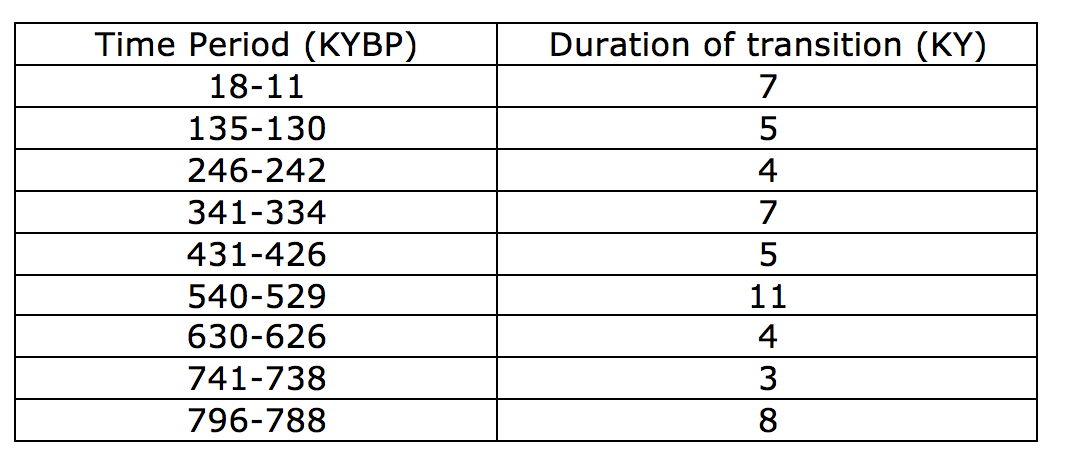
Reviewing all the data as far back as 8000,000 years, the durations required for the termination ramp from glacial to interglacial conditions in the last nine deglaciations are listed in Table 1. On average, the duration of the transition from glacial to deglacial conditions took roughly 6,000 years (about ¼ of a precessional period).
Table 1. Durations required for the transition from glacial to interglacial conditions.
Variation of physical variables through the termination cycle
Data on the patterns of the transition from glacial maximum to termination ramp to Interglacial are shown in Figures 3 to 5.
Figure 3. Superposition of nine temperature curves around the last termination (WAIS, 2013).
Figure 4. Temperature change through the current Interglacial. (Masson-Delmotte et al.(2011))
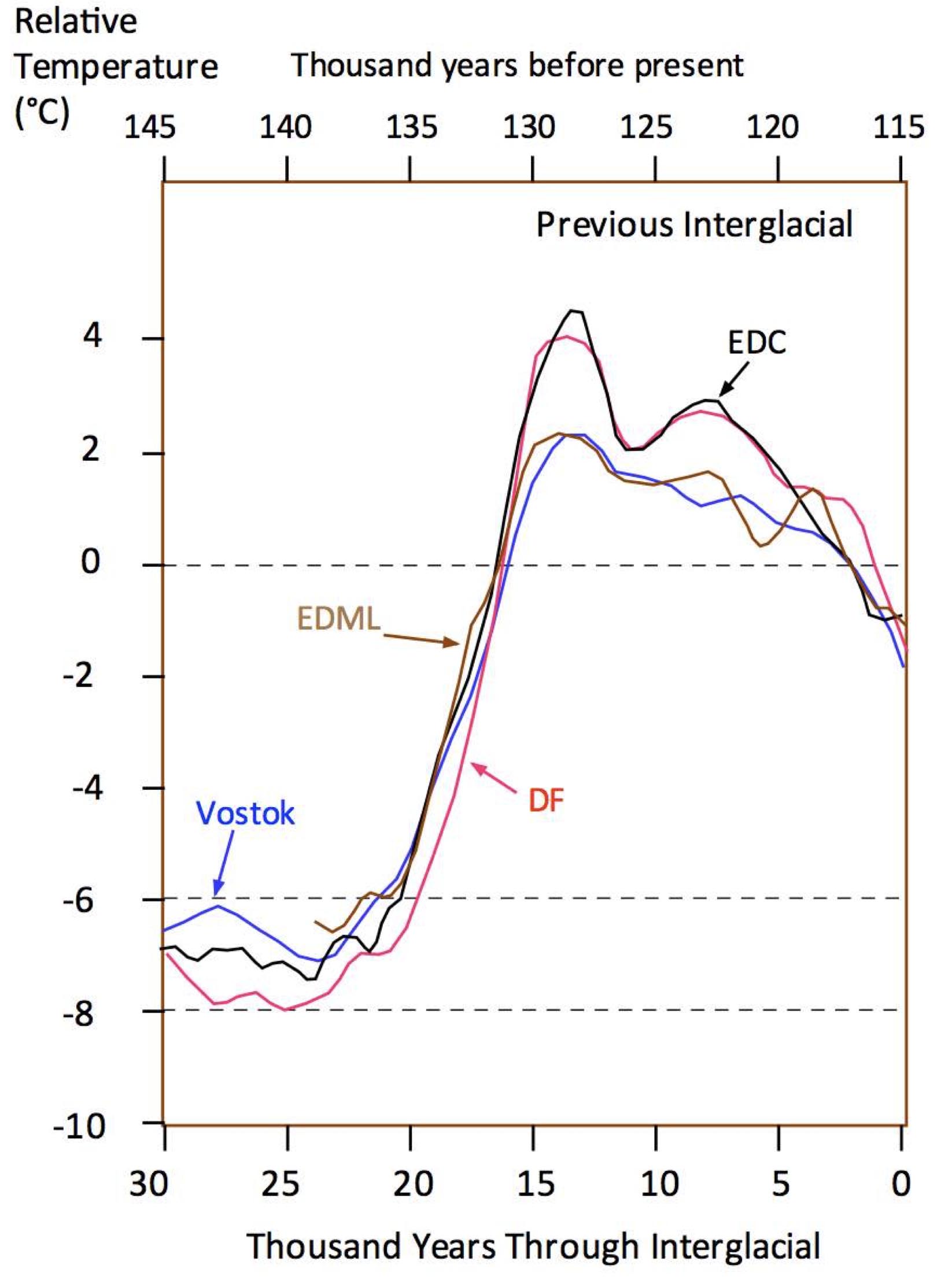
Figure 5. Temperature change before and through the previous Interglacial. (Masson-Delmotte et al.(2011))
It has been found that sharply rising dust levels preceded termination in every case over the last 800,000 years. Data on the last two terminations are given in Figure 6.
Figure 6. Comparison of dust deposition rate and temperature change through the last and previous terminations. Dust data from Schneider et al.(2013). Temperature data from Masson-Delmotteet al.(2011)or WAIS (2013).
Dust deposition as a trigger to initiate terminations of Ice Ages
Ellis and Palmer (2016)emphasized the importance of dust deposition as a trigger to initiate terminations of Ice Ages.
As Ellis put it (private communication):
“Almost everyone agreed that Milankovitch cycles controlled the glacial cycle. But they were unable to explain why some cycles failed to produce an interglacial while others did, and during subsequent research it became apparent that there was no accepted answer to this troubling but central question. A theory is not a theory, if it has a thumping great lacuna in the middle of it. This led me into a detailed study of the glacial cycle, and the revelation dust was at a peak just before each interglacial.
It was only when Michael Palmer sought to refine my rough and rugged draft paper, that the prior research of Mahowald and Ganopolski and many others was discovered. And it was surprising that all of these papers danced around what I saw as the central agent of Ice Age modulation, without identifying and explaining it as such. Ganopolski, for instance, identified a link between ice sheet volume and dust and presumed that the volume of ice was causing the dust – in other words this must have been glaciogenic dust caused by ice-rock erosion. But previous papers had already identified the source of the dust as the Gobi and Taklamakan deserts, excluding the possibility that the dust was glaciogenic.”
Ellis and Palmer (2016)said:
“When CO2reaches a minimum and albedo reaches a maximum [at the peak of an Ice Age], the world rapidly warms into an interglacial. A similar effect can be seen at the peak of an interglacial, where high CO2and low albedo results in cooling. This counterintuitive response of the climate system also remains unexplained, and so a hitherto unaccounted-for agent must exist that is strong enough to counter and reverse the classical feedback mechanisms.”
They proposed:
The answer to both of these conundrums lies in glacial dust, which was deposited upon the ice sheets towards the end of each glacial maximum… during the glacial maximum, CO2depletion starves terrestrial plant life of a vital nutrient and causes a die-back of upland forests and savannahs, resulting in widespread desertification and soil erosion. The resulting dust storms deposit large amounts of dust upon the ice sheets and thereby reduce their albedo, allowing a much greater absorption of insolation.
They asserted that their proposal:
… explains each and every facet of the glacial cycle, and all of the many underlying mechanisms that control its periodicity and temperature excursions and limitations.
The paper by Ellis and Palmer then discussed variability of solar input to high latitudes, which is very heavily traveled ground, and we need not elaborate on this here. But one point they raised is worth emphasizing: One cannot invoke rising solar input to high latitudes as the sole cause of terminations of Ice Ages since many such increases in solar input do not produce terminations. Increased solar input might be necessary for terminations but it is clearly not sufficient.
The theory of Ellis and Palmer explains how terminations occur, but it does not necessarily explain why Interglacials terminate. Once an Interglacial is established, history shows that that a new Ice Age typically begins in less than ten thousand years. A likely explanation for this, as an addendum to the theory of Ellis and Palmer, is to note that during the course of an Interglacial, CO2rises rapidly toward about 280 ppm, the plant life of the Earth resuscitates, and dust levels drop precipitously. While the ice sheets are greatly reduced from the levels of the Ice Age, substantial amounts of remnant snow and ice remain at high latitudes. Lacking dust on these ice sheets, the energy balance favors expansion of the ice sheets. The 11,000-year up-lobe in solar input to high altitudes that coincided with the termination and Interglacial now turns sharply downward, thus supporting expansion of the ice sheets as the outcome of the Interglacial. A nascent new Ice Age begins. This Ice Age continues for up to about 100,000 years until the CO2concentration drops so far that plant life is severely affected, dust becomes prevalent, and the cycle continues.
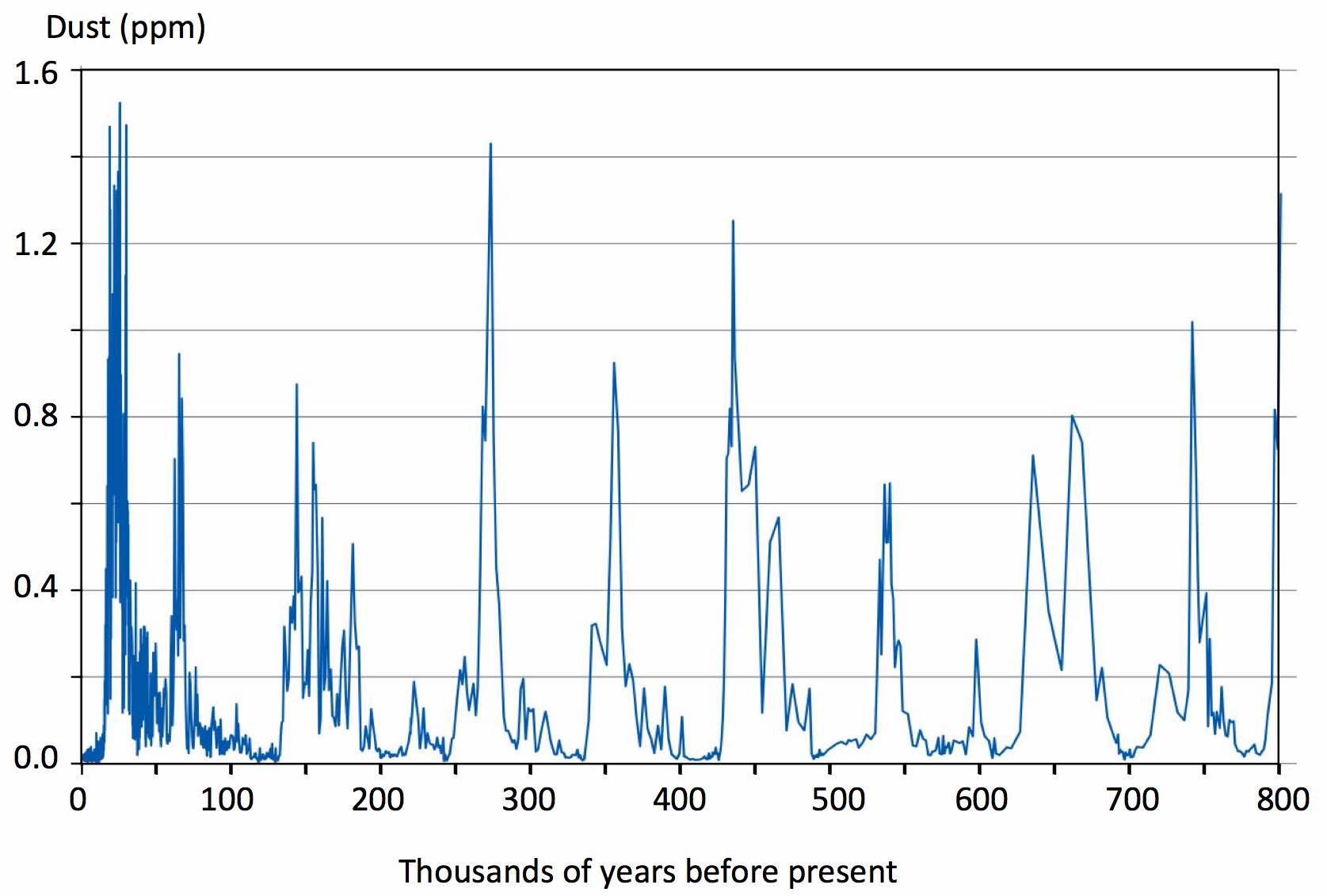
Measured dust levels in Antarctic ice cores are summarized in Figures 7 and 8, using the Coulter method and the laser method.
Figure 7. Antarctic dust concentration in ice cores as measured by the Coulter method. (Lambert, et al.(2008))
Figure 8. Antarctic dust concentration in ice cores as measured by a laser optical method. (Lambert, et al.(2008))
The essential basis for the hypothesis advanced by Ellis and Palmer is illustrated in Figures 9 and 10. The lower graph in these figures shows the dust loading in the ice core at Antarctica. The middle graph shows peak solar intensity at 65°N on June 21. The top graph shows the Antarctic temperature anomaly. Vertical red dashed lines are drawn at each major sharp rise in Antarctic temperature, presumably initiating a termination.
From the data, we immediately observe:
- Sharp dust peaks and/or dust accumulations immediately precede all terminations.
- Up-swings of the oscillatory solar intensity occur at the start of each termination.
The inevitable conclusion must be:
Terminations are essentially always preceded by a buildup of dust and mainly occur on a sharply rising lobe of the solar oscillation.
Therefore, the inference made by Ellis and Palmer is that two situations are necessary precursors to a termination of an Ice Age:
(1) There must be a sharp maximum in dust loading. (But this typically occurs after there has been a long, extended Ice Age).
(2) The sharp dust maximum must coincide with sharply rising solar intensity.
Note particularly that sharply rising solar input to high latitudes by itself does not necessarily lead to a termination. Many such high amplitude lobes of solar input to high latitudes do not lead to termination. Termination only occurs with rising solar input to high latitudes, after reaching the depth of the greatest CO2reduction in a very mature Ice Age, combined with peak dust. Most high amplitude lobes of solar input to high latitudes have only moderate effect on the growth of ice sheets. Therefore, one might infer that peak dust is even more important than solar input to high latitudes in termination of Ice Ages. While these inferences do not in themselves prove a cause–effect relationship, they are highly suggestive.
Figure 9. (top) Antarctic temperature. (middle) Solar intensity at 65°N on June 21. (bottom) Dust loading in Antarctica ice core using the Coulter counter.
Figure 10. (top) Antarctic temperature. (middle) Solar intensity at 65°N on June 21. (bottom) Dust loading in Antarctica ice core using the laser counter.
Dust fluxes at LGM and solar absorption
Lambert et al.(2015) presented a new global dust flux data set for Holocene and LGM based on observational data. They created a new interpolation of the unevenly spaced Holocene and LGM dust flux measurements compiled in the DIRTMAP database to two global grids. As in most studies, they were primarily interested in the impact of enhanced glacial oceanic iron deposition on the LGM-Holocene carbon cycle, rather than dust deposition on ice sheets. The only place where any information was provided for deposition at Greenland or North America during the LGM was in a small color-coded map with rather crude resolution. A rough reading of this map indicated the rates of deposition of dust as follows:
Greenland (core drilling region) 0.3 g/m2/yr
Greenland (southern tip) 0.8 g/m2/yr
Great Lakes area: 32 g/m2/yr
Laurentide ice sheet: 12 g/m2/yr
Maher et al.(2010)and Lambert et al.(2015) made estimates of dust deposition rates for the Laurentide ice sheet and the Great Lakes area at the LGM. An average of these values is:
Great Lakes area: 20 g/m2/yr
Laurentide ice sheet: 7 g/m2/yr
Following Mahowaldet al.(1999), it is assumed that the average diameter of a dust particle is 2.5 microns. The geometrical blocking area of a dust particle is therefore estimated to be
3.14 ´(1.25 ´10-6)2m2~ 5 ´10-12m2.
And the mass of a dust particle is estimated to be
4/3 ´3.14 ´(1.25 ´10-6)3m3´1.5 ´106 g/m3= 1.2 ´10-11 g
Based on purely geometrical effects, the geometrical blocking area of surface dust is estimated to be:
5 ´10-12m2/ 1.2 ´10-11 g = 0.4 m2of blocking area per g/m2of dust
Hence in the geometrical approximation, a layer of 2.5 g/m2of surface dust completely blocks a surface optically. A layer of 1 g/m2of surface dust blocks 40% of the surface.
The above estimates are based on geometry, treating a dust particle as a sphere of diameter 2.5 microns. However, the effective cross-sectional area of a particle for light scattering and absorption, Asis related to the geometrical area of a particle, Ad, by the relation:
As= AdQext
where Qextis the so-called extinction efficiency or scattering efficiency. It turns out that because of diffraction effects, Qextis >1. In analyzing dust on Mars, Tomasko (1999)estimated Qext~ 2.6. Thus, the true optical effect of 1 g/m2of dust particles is to optically block 100% of the surface. Mars dust is roughly similar to Earth dust in regard to average diameter.[2]
When light interacts with a single particle, some light can be scattered into the forward cone, some light can be scattered into the backward cone, and some light can be absorbed. According to studies of Mars dust, the best estimate is that of the total amount of light scattered and absorbed, 7% is absorbed, 77% is forward-scattered, and 16% is back-scattered. Note that most of the scattering is in the forward direction. Thus, the predominant effect of dust particles embedded in ice is to forward scatter the light deeper into the ice and to a lesser extent, absorb the light.
Source of the dust
Ellis and Palmer (2016)reviewed at length, data and models on the source of dust and albedo effects of dust during Ice Ages. I will be content with only a very brief mention of only a few points they raised. There seems little doubt that the combination of low temperature and low CO2at the LGM was detrimental to plant life. They argued that the principal impact was on high altitude regions, normally arid regions, and northern regions during summer. The source determined by isotopic analysis was attributed to the Gobi and Taklamakan deserts, and there was little evidence of glaciogenic dust. As Ellis put it (private communication):
The question is how these peaks in dust flux were generated during the latter millennia of each Ice Age. If it was not the grinding of ice sheets that caused the dust, then what did? The likely answer was that the low CO2concentrations at each glacial maximum led to plant extinction in high altitude arid regions, turning them into new CO2deserts. And this was a scenario that fitted the source region for Greenland dust very well – the Gobi. The Gobi is mostly steppe grassland, but under the low CO2conditions of a glacial maximum the entire Gobi became a shifting-sand desert that created vast dust clouds, as is proven by the massive dust deposits upon the Loess Plateau in China.
And so, the beauty of this theory … is that it is a simple thought-experiment that can be followed by anyone, and yet in my view it explains every facet of the glacial-interglacial cycle. And it even explains the previously inexplicable – the reason why some strong precessional insolation maxima failed to produce much in the way of melting and warming, let alone an Interglacial.
In short:
Ice Ages cause ice sheet extension Þoceanic cooling Þoceanic CO2absorption = plant asphyxiation on the Gobi plateau Þnew CO2deserts Þdust generation Þice sheet contamination for 10 kyrs.
Then:
Rising NH Milankovitch insolation Þice sheet surface ablation and melting Þice sheet dust exposure and concentration Þice sheet albedo reduction Þincreased insolation absorption Þincreased ablation and melting ÞInterglacial.
It is a simple feedback system that is very powerful and operates regionally, unlike CO2which is a global feedback agent of indeterminate strength. And yet we know that Interglacials are regional phenomena rather than global phenomena, because they only coincide with increased Milankovitch insolation in the northern hemisphere, and never with increased insolation in the south. Ergo, the primary feedback controlling interglacial inception must be regional to the NH, rather than global.
Summary
I think that Ellis makes some powerful arguments here; yet uncertainties remain about how much dust was deposited at the LGM and how effective that dust was in increasing the absorptivity of the ice sheets. The Antarctic data support the hypothesis but Antarctica is a long way from the ice sheets. The Greenland data are more enigmatic. It is widely agreed that dust deposition on the ice sheets was much greater than it was at Greenland or Antarctica, but so was the rate of snow accumulation.
The hypothesis put forth by Ellis and Palmer has considerable potential merit. As the Ice Age deepens, the combination of low CO2levels, cold, and wind turns originally marginal, semi-desert regions into major sources of wind-blown dust. The evidence from ice cores indicates that the LGM was a period with relatively high levels of atmospheric dust blown by strong winds. Some models estimate relatively high levels of dust deposition on the ice sheets at the LGM. These levels of dust deposition would significantly darken the upper levels of the ice sheets. Thus, as Ellis and Palmer suggested, dust levels on the ice sheets peaked prior to and at the LGM, providing a mechanism to initiate a termination when synchronized with an up-lobe in summer solar input to high northern latitudes. The role of dust in terminations of Ice Ages is probably far more important than many realize. It appears likely that unusually high dust levels coupled to sharply rising solar intensity at high latitudes was a major factor in initiating termination of Ice Ages. However, as always in such speculations, uncertainties remain.
Finally, it is noteworthy that because Ellis and Palmer (2016)was published in an obscure journal, it seems to have been somewhat ignored by the science community. My hope is that my book will give their theory additional exposure.
Bonehead model for Ice Ages:
In the following, I propose a modification to the Paillard (1998)model.
I hypothesize four states of the Earth system:
I= interglacial
g= mild glacial
G= glacial maximum
U= termination
Each of these is characterized by an ice volume parameter vRand a time constant for ice volume change, TR, where subscript Rcan be I, g, Gor U. At any time t, v= the current ice volume and dv/dt = rate of change of ice volume.
There is a constantly acting solar forcing term F(t) with amplitude that oscillates with the precession frequency. The time starts at some negative value (years) and works its way forward via integration of differential equations. We can gain insight into the magnitudes of the vRas follows.
The basic equation is
dv/dt = (vR– v)/TR– F(t)
in which the rate of change of ice volume in any state of the system is a maximum when v is small and is a minimum when vis large. The solar forcing term F(t) oscillates with a ~22,000 year period due to precession. F(t) is measured from its average, so it can be negative or positive.
When the first term on the right side is large (v<< vR), the first term outweighs F(t) and the ice sheets are growing. As F(t) oscillates, it can add or subtract from the first term’s contribution to dv/dt, but dv/dt remains substantial. This is the “g” state.
After passing through the “g” state for about four periods of precession (roughly 90,000 years), vreaches a level that we characterize as the “LGM” or in this model, the “G” state. In the “G” state, the first term becomes small compared to F(t). As long as F(t) remains in a down-lobe (about 11,000 years) the “G” state persists. But when F(t) enters an up-lobe, dv/dt turns negative and the system enters the “U” state – termination. The “U” state persists for about half of the up-lobe, and when most of the ice is gone (in about 5,500 years), the system enters the “I” state – an Interglacial – during which the ice volume remains low but does not change. The Interglacial lasts another 5,500 years as the solar up-lobe diminishes. Finally, F(t) enters a down-lobe and dv/dt turns positive and a new “g” state begins.
Figure 11shows a simplistic picture of the variation of vand dv/dtwith t. In the plot of dv/dt vs. t, the area under the curve in the “g” region must equal the area of the rectangle in the “U” region (to conserve mass). Figure 11does not show the effect of variation of insolation. In region “g”, up-lobes and down-lobes of solar due to precession add ups and downs to the smooth curve shown.
Figure 11. Schematic variation of vand dv/dt vs. t.
Consider a system at t= 0 early in the Interglacial state. We require that v< vIand F(t)is large enough that dv/dtis slightly less than 0.
dv/dt = (vI– v)/TI– F(t)is slightly less than zero at start of “I” state with F(t)on an up-lobe of precession.
Furthermore, the magnitudes must be chosen such that when F(t)heads downward due to precession, a point will be reached where dv/dtturns positive. At that point, the system switches to the “g” state.
Now the system switches to a new differential equation:
dv/dt = (vg– v)/Tg– F(t)
Here, vgis large, so that the rate of buildup of ice volume remains > 0 throughout. However, as v builds up, the rate of accumulations decreases. Furthermore, the ups and downs of F(t)due to precession adds up and down perturbations to the progress of the ever increasing ice volume.
At some point in time, when vgets large enough, the system switches to the “G” state. It is not clear a priori how to set this transition. Perhaps when v reaches say, 90% of vg? At such a point, the rate of accumulation has slowed down considerably and the ice volume is large. In the “G” state,
dv/dt = (vG– v)/TG– F(t)
The parameters must be chosen so that dv/dt ~ 0 for moderate F(t). At some point, an up-lobe in the precession cycle occurs, and F(t) increases. When dv/dtturns positive, the system enters the “U” state. In the “U” state:
dv/dt = (vU– v)/TU– F(t)
Here, dv/dt << 0 and the system undergoes a rapid termination. When v reaches a critically small level, the system enters the “I” state and the cycle begins over again. Determining appropriate values (and units) of the parameters is likely to be a tricky business. It seems likely that vU~ vG~ vgare large whereas vIis small. Clearly, TUmust be the smallest time parameter.
Figure 12illustrates the theory further. Note that in actuality, the amplitude of the solar oscillations varies from cycle to cycle but they are drawn in the figure (for simplicity) as if the amplitude never changes. Figures 11 and 12 are highly idealized, and each glacial-interglacial cycle will have its own unique character. Ups and downs (as illustrated by the blue curves) might be quite different in reality from this idealized picture of events.
Figure 12. Schematic representation of (dv/dt) in the transitions to and from Ice Ages.
In this model, there are four periods within the Ice Age cycles. The “g” period (white background) involves long-term buildup of the ice sheets over many decades. In this glacial period, the rate of accumulation decreases with time. After about 4 solar precessional cycles (~88,000 years), the ice sheets approach their greatest extent. The system then enters the “G” state – a global ice maximum (brown background). This global glacial maximum lasts for about 11,000 years, and occurs during a solar down-lobe, and the CO2concentration drops to its lowest level (less than 200 ppm). This impacts plant life, and heavy dust deposition occurs on the ice sheets. With the next solar up-lobe, the combination of heavy dusting and rising solar intensity produces a termination (“U” state – green background). The ice sheets dissipate in a mere ~5,500 years. As termination proceeds, the CO2concentration rises, plant life recovers, and dust levels drop precipitously. When the ice sheets reach a minimum, the system enters the Interglacial state (“I”) (blue background) which lasts another ~5,500 years, completing the solar up-lobe. The Interglacial state has a climate not unlike that of today. When the solar curve turns downward, the value of dv/dt turns positive and a new Ice Age begins (“g” state begins anew). The total length of the “U” and “I” states is ~11,000 years.
The black curve in Figure 12shows a simplified dv/dt (where v is the total ice volume) neglecting solar variations. The solar cycle relentlessly oscillates with the ~22,000 period due to precession. The blue curve shows the effect of solar perturbations on dv/dt. Each up-lobe and down-lobe produces a corresponding “bump” in the dv/dt curve but a termination cannot ensue until the “G” state, when dust deposition decreases the albedo of the ice sheets.
Figure 13shows the corresponding curves for ice volume v(t). In this model, the variability of the solar input to high latitudes is inconsequential during the long-lasting “g” state. In the “g” state, dv/dt is dominated by the first term on the right side of the equation. The Solar input comes into play only near the end of an Ice Age. The amplitude of the solar oscillations (due to precession) is not important; only the phasing matters. A down-lobe in solar late in the Ice Age produces a glacial maximum. During that time, CO2sinks to its lowest values and large amounts of dust are generated and transported by winds. As the precessional cycle turns upward, a termination sets in. An Interglacial follows until precession drives the solar curve downward. Solar precession acts as the pacemaker for transitions from gto Gto Uto Ito g.
Figure 13. Schematic representation of v(t)in the transitions to and from Ice Ages.
While the models as shown in Figures 12 and 13are very satisfying in their simplicity, nature is not so cooperative. This simple picture does not adequately describe the reality in detail, although it does have some characteristics that resemble reality in very rough outline.
Addendum
This write-up is abstracted from chapters 8 and 11 of the third edition of my book on Ice Ages which is now in press and might be available in early 2019. I am willing to send pdf versions of the chapters to serious scientists on request.
References
Ellis, Ralph and Michael Palmer (2016) “Modulation of Ice Ages via precession and dust-albedo feedbacks” Geoscience Frontiershttp://www.sciencedirect.com/science/article/pii/S1674987116300305
Lambeck, Kurt et al.(2014) “Sea level and global ice volumes from the Last Glacial Maximum to the Holocene” PNAS111, 15296–15303.
Lambert, F. et al.(2008) “Dust-climate couplings over the past 800,000 years from the EPICA Dome C ice core” Nature452, 616-619
Lambert, Fabrice (2015) “Dust fluxes and iron fertilization in Holocene and Last Glacial Maximum climates” Geophys. Res. Lett.,42, 1-10.
Maher, Barbara et al.(2010) “Global connections between Aeolian dust, climate and ocean biogeochemistry at the present day and at the last glacial maximum” Quaternary Science Reviews99, 61-97.
Mahowald, N.et al.(1999) “Dust sources and deposition during the last glacial maximum and current climate: A comparison of model results with paleodata from ice cores and marine sediments” JGR104, 15895-15916.
Masson-Delmotteet al.(2011) “A comparison of the present and last interglacial periodsin six Antarctic ice cores” Clim. Past7, 397–423.
Paillard, Didier (1998) “The timing of Pleistocene glaciations from a simple multiple-state climate model,” Nature 391, 378-381.
Rothlisberger, R., M. et al.(2008) ‘‘The southern hemisphere at glacial terminations: Insights from the Dome C ice core,’’ Climate of the Past Discussions, 4, 761–789.
WAIS (2013) “Onset of deglacial warming in West Antarctica driven by local orbital forcing”Nature500, 440-446.
Wolff, E. W.et al.(2016) “Interglacials of the past 800,000 years” Past Interglacials Working Group of Interglacials of the last 800,000 years, Reviews of Geophysics54, 162–219.
[1]https://scienceofdoom.com/2014/04/14/ghosts-of-climates-past-nineteen-ice-sheet-models-i/
[2]Rapp, D. Human missions to Mars, 2ndedition, Springer-Verlag, 2016.
Moderation note: As with all guest posts, please keep your comments civil and relevant.