by Nic Lewis
A critique of a recent paper by Brown and Caldeira published in Nature that predicted greater than expected global warming.
Last week a paper predicting greater than expected global warming, by scientists Patrick Brown and Ken Caldeira, was published by Nature.[1] The paper (henceforth referred to as BC17) says in its abstract:
“Across-model relationships between currently observable attributes of the climate system and the simulated magnitude of future warming have the potential to inform projections. Here we show that robust across-model relationships exist between the global spatial patterns of several fundamental attributes of Earth’s top-of-atmosphere energy budget and the magnitude of projected global warming. When we constrain the model projections with observations, we obtain greater means and narrower ranges of future global warming across the major radiative forcing scenarios, in general. In particular, we find that the observationally informed warming projection for the end of the twenty-first century for the steepest radiative forcing scenario is about 15 per cent warmer (+0.5 degrees Celsius) with a reduction of about a third in the two-standard-deviation spread (−1.2 degrees Celsius) relative to the raw model projections reported by the Intergovernmental Panel on Climate Change.”
Patrick Brown’s very informative blog post about the paper gives a good idea of how they reached these conclusions. As he writes, the central premise underlying the study is that climate models that are going to be the most skilful in their projections of future warming should also be the most skilful in other contexts like simulating the recent past. It thus falls within the “emergent constraint” paradigm. Personally, I’m doubtful that emergent constraint approaches generally tell one much about the relationship to the real world of aspects of model behaviour other than those which are closely related to the comparison with observations. However, they are quite widely used.
In BC17’s case, the simulated aspects of the recent past (the “predictor variables”) involve spatial fields of top-of-the-atmosphere (TOA) radiative fluxes. As the authors state, these fluxes reflect fundamental characteristics of the climate system and have been well measured by satellite instrumentation in the recent past – although (multi) decadal internal variability in them could be a confounding factor. BC17 derive a relationship in current generation (CMIP5) global climate models between predictors consisting of three basic aspects of each of these simulated fluxes in the recent past, and simulated increases in global mean surface temperature (GMST) under IPCC scenarios (ΔT). Those relationships are then applied to the observed values of the predictor variables to derive an observationally-constrained prediction of future warming.[2]
The paper is well written, the method used is clearly explained in some detail and the authors have archived both pre-processed data and their code.[3] On the face of it, this is an exemplary study, and given its potential relevance to the extent of future global warming I can see why Nature decided to publish it. I am writing an article commenting on it for two reasons. First, because I think BC17’s conclusions are wrong. And secondly, to help bring to the attention of more people the statistical methodology that BC17 employed, which is not widely used in climate science.
What BC17 did
BC17 uses three measures of TOA radiative flux: outgoing longwave radiation (OLR), outgoing shortwave radiation (OSR) – being reflected solar radiation – and the net downwards radiative imbalance (N).[4] The aspects of each of these measures that are used as predictors are their climatology (the 2001-2015 mean), the magnitude (standard deviation) of their seasonal cycle, and monthly variability (standard deviation of their deseasonalized monthly values). These are all cell mean values on a grid with 37 latitudes and 72 longitudes, giving nine predictor fields each with 2664 values for three aspects (climatology, seasonal cycle and monthly variability) for each of three variables (OLR, OSR and N). So, for each climate model there are up to 23,976 predictors of GMST change.
BC17 consider all four IPCC RCP scenarios and focus on mid-century and end-century warming; in each case there is a single predictand, ΔT . They term the ratio of the ΔT predicted by their method to the unweighted mean of the ΔT values actually simulated by each of the models involved the ‘Prediction ratio’. They assess the predictive skill as the ratio of the root-mean-square error of the differences for each model between its predicted ΔT and its actual (simulated) ΔT, to the standard deviation of the simulated changes across all the models. They call this the Spread ratio. For this purpose, each model’s predicted ΔT is calculated using the relationship between the predictors and ΔT determined using only the remaining models.[5]
As there are more predictors than data realizations (with each CMIP5 model providing one realization), using them directly to predict ΔT would involve massive over-fitting. The authors avoid over-fitting by using a partial least squares (PLS) regression method. PLS regression is designed to compress as much as possible of the relevant information in the predictors into a small number of orthogonal components, ranked in order of (decreasing) relevance to predicting the predictand(s), here ΔT. The more PLS components used, the more accurate the in-sample predictions will be, but beyond some point over-fitting will occur. The method involves eigen-decomposition of the cross-covariance, in the set of models involved, between the predictors and ΔT. It is particularly helpful when there are a large number of collinear predictors, as here. PLS is closely related to statistical techniques such as principal components regression and canonical correlation analysis. The number of PLS components to retain is chosen having regard to prediction errors estimated using cross-validation, a widely-used technique.[6] BC17 illustrates use of up to ten PLS components, but bases its results on using the first seven PLS components, to ensure that over-fitting is avoided.
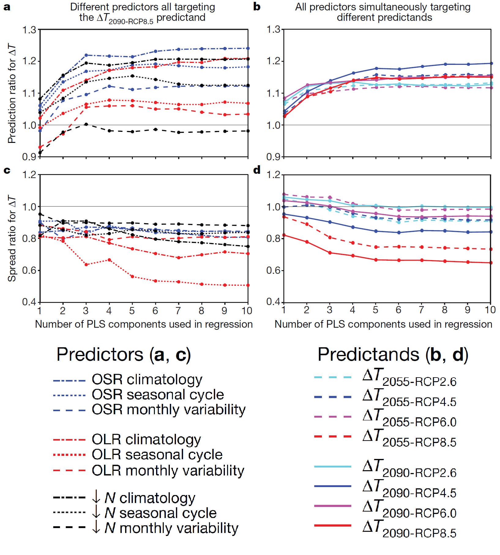
The main result of the paper, as highlighted in the abstract, is that for the highest-emissions RCP8.5 scenario predicted warming circa 2090 [7] is about 15% higher than the raw multimodel mean, and has a spread only about two-thirds as large as that for the model-ensemble. That is, the Prediction ratio in that case is about 1.15, and the Spread ratio is about 2/3. This is shown in their Figure 1, reproduced below. The left hand panels all involve RCP8.5 2090 ΔT as the predictand, but with the nine different predictors used separately. The right hand panels involve different predictands, with all predictors used simultaneously. The Prediction ratio and Spread ratio for the main results RCP8.5 2090 ΔT case highlighted in the abstract is shown by the solid red line in panels b and d respectively, at an x-axis value of 7 PLS components.
Figure 1. Sensitivity of results to predictors or predictands used and to the number of PLS components used. a, Prediction ratios for the nine predictor fields, each individually targeting the ΔT 2090-RCP8.5 predictand. b, As in a but using all nine of the predictor fields simultaneously while switching the predictand that is targeted. c, d As in a, b respectively but showing the Spread ratios using hold-one-out cross-validation.
Is there anything to object to in this work, leaving aside issues with the whole emergent constraint approach? Well, it seems to me that Figure 1 shows their main result to be unsupportable. Had I been a reviewer I would have recommended against publishing, in the current form at least. As it is, this adds to the list of Nature-brand journal climate science papers that I regard as seriously flawed.
Where BC17 goes wrong, and how to improve its results
The issue is simple. The paper is, as it says, all about increasing skill: making better projections of future warming with narrower ranges by constraining model projections with observations. In order to be credible, and to narrow the projection range, the predictions of model warming must be superior to a naïve prediction that each model’s warming will be in line with the multimodel average. If that is not achieved – the Spread ratio is not below one – then no skill has been shown, and therefore the Prediction ratio has no credibility. It follows that the results with the lowest Spread ratio – the highest skill – are prima facie most reliable and to be preferred.
Figure 1 provides an easy comparison between different predictors of skill in predicting ΔT for the RCP8.5 2090 case. That case, as well as being the one dealt with in the paper’s abstract, involves the largest warming and as a result the highest signal to noise ratio. Moreover, it has data for nearly all the models (36 out of 40). Accordingly, RCP8.5 2090 is the ideal case for skill comparisons. Henceforth I will be referring to that case if not stated otherwise.
Panel d shows, as the paper implies, that use of all the predictors results in a Spread ratio of about 2/3 with 7 PLS components. The Spread ratio falls marginally to 65% with 10 PLS components. The corresponding Prediction ratios are 1.137 with 7 components and 1.141 with 10 components. One can debate how many PLS components to retain, but it makes very little difference whether 7 or 10 are used and 7 is the safer choice. The 13.7% uplift in predicted warming in the 7 PLS components case used by the authors is rather lower than the “about 15%” stated in the paper, but no matter.
The key point is this. Panel c shows that using just the OLR seasonal cycle predictor produces a much more skilful result than using all predictors simultaneously. The Spread ratio is only 0.53 with 7 PLS components (0.51 with 10). That is substantially more skilful than when using all the predictors – a 40% greater reduction below one in the Spread ratio. Therefore, the results based on just the OLR seasonal cycle predictor must be considered to be more reliable than those based on all the predictors simultaneously.[8] Accordingly, the paper’s main results should have been based on them in preference to the less skilful all-predictors-simultaneously results. Doing so would have had a huge impact. The RCP8.5 2090 Prediction ratio using the OLR seasonal cycle predictor is under half that using all predictors – it implies a 6% uplift in projected warming, not “about 15%”.
Of course, it is possible that an even better predictor, not investigated in BC17, might exist. For instance, although use of the OLR seasonal cycle predictor is clearly preferable to use of all predictors simultaneously, some combination of two predictors might provide higher skill. It would be demanding to test all possible cases, but as the OLR seasonal cycle is far superior to any other single predictor it makes sense to test all two-predictor combinations that include it. I accordingly tested all combinations of OLR seasonal cycle plus one of the other eight predictors. None of them gave as high a skill (as low a Spread ratio) as just using the OLR seasonal cycle predictor, but they all showed more skill than the use of all three predictors simultaneously, save to a marginal extent in one case.
In view of the general pattern of more predictors producing a less skilful result, I thought it worth investigating using just a cut down version of the OLR seasonal cycle spatial field. The 37 latitude, 72 longitude grid provides 2,664 variables, still an extraordinarily large number of predictors when there are only 36 models, each providing one instance of the predictand, to fit the statistical model. It is thought that most of the intermodel spread in climate sensitivity, and hence presumably in future warming, arises from differences in model behaviour in the tropics.[9] Therefore, the effect of excluding higher latitudes from the predictor field seemed worth investigating.
I tested use of the OLR seasonal cycle over the 30S–30N latitude zone only, thereby reducing the number of predictor variables to 936 – still a large number, but under 4% of the 23,976 predictor variables used in BC17. The Spread ratio declined further, to 51% using 7 PLS components.[10] Moreover, the Prediction ratio fell to 1.03, implying a trivial 3% uplift of observationally-constrained warming.
I conclude from this exercise that the results in BC17 are not supported by a more careful analysis of their data, using their own statistical method. Instead, results based on what appears to be the most appropriate choice of predictor variables – OLR seasonal cycle over 30S–30N latitudes – indicate a negligible (3%) increase in mean predicted warming, and on their face support a greater narrowing of the range of predicted warming.
For possible reasons for the problems with BC17’s application of PLS regression, see the longer and more detailed post at ClimateAudit.
Why BC17’s results would be highly doubtful even if their application of PLS were sound
Despite their superiority over BC17’s all-predictors-simultaneously results, I do not think that revised results based on use of only the OLR seasonal cycle predictor, over 30S–30N, would really provide a guide to how much global warming there would actually be late this century on the RCP8.5 scenario, or any other scenario. BC17 make the fundamental assumption that the relationship of future warming to certain aspects of the recent climate that holds in climate models also applies in the real climate system. I think this is an unfounded, and very probably invalid, assumption. Therefore, I see no justification for using observed values of those aspects to adjust model-predicted warming to correct model biases relating to those aspects, which is in effect what BC17 does.
Moreover, it is not clear that the relationship that happens to exist in CMIP5 models between present day biases and future warming is a stable one, even in global climate models. Webb et al (2013),9 who examined the origin of differences in climate sensitivity, forcing and feedback in the previous generation of climate models, reported that they “do not find any clear relationships between present day biases and forcings or feedbacks across the AR4 ensemble”.
Furthermore, it is well known that some CMIP5 models have significantly non-zero N (and therefore also biased OLR and/or OSR) in their unforced control runs, despite exhibiting almost no trend in GMST. Since a long-term lack of trend in GMST should indicate zero TOA radiative flux imbalance, this implies the existence of energy leakages within those models. Such models typically appear to behave unexceptionally in other regards, including as to future warming. However, they will have a distorted relationship between climatological values of TOA radiative flux variables and future warming that is not indicative of any genuine relationship between them that may exist in climate models, let alone of any such relationship in the real climate system.
There is yet a further indicator that the approach used in the study tells one little even about the relationship in models between the selected aspects of TOA radiative fluxes and future warming. As I have shown, in CMIP5 models that relationship is considerably stronger for the OLR seasonal cycle than for any of the other predictors or any combination of predictors. But it is well established that the dominant contributor to intermodel variation in climate sensitivity is differences in low cloud feedback. Such differences affect OSR, not OLR, so it would be surprising that an aspect of OLR would be the most useful predictor of future warming if there were a genuine, underlying relationship in climate models between present day aspects of TOA radiative fluxes and future warming.
Conclusion
To sum up, I have shown strong evidence that this study’s results and conclusions are unsound. Nevertheless, the authors are to be congratulated on bringing the partial least squares method to the attention of a wide audience of climate scientists, for the thoroughness of their methods section and for making pre-processed data and computer code readily available, hence enabling straightforward replication of their results and testing of alternative methodological choices.
Endnotes
[1] Greater future global warming inferred from Earth’s recent energy budget, doi:10.1038/nature24672. The paper is pay-walled but the Supplementary Information, data and code are not.
[2] Uncertainty ranges for the predictions are derived from cross-validation based estimates of uncertainty in the relationships between the predictors and the future warming. Other sources of uncertainty are not accounted for.
[3] I had some initial difficulty in running the authors’ Matlab code, as a result of only having access to an old Matlab version that lacked necessary functions, but I was able to adapt an open source version of the Matlab PLS regression module and to replicate the paper’s key results. I thank Patrick Brown for assisting my efforts by providing by return of email a missing data file and the non-standard color map used.
[4] N = incoming solar radiation – OSR – OLR; with OSR and OLR being correlated, there is only partial redundancy in also using the derived measure N.
[5] That is, (RMS) prediction error is determined using hold(leave)-one-out cross-validation.
[6] For each CMIP5 model, ΔT is predicted based on a fit estimated with that model excluded. The average of the squared resulting prediction errors will start to rise when too many PLS components are used.
[7] Average over 2081-2100.
[8] Although I only quote results for the RCP8.5 2090 case, which is what the abstract covers, I have checked that the same is also true for the RCP4.5 2090 case (a Spread ratio of 0.66 using 7 PLS components, against 0.85 when using all predictors). In view of the large margin of superiority in both cases it seems highly probable that use of the OLR seasonal cycle produces more skilful predictions for all predictand cases.
[9] Webb, M J et al 2013: Origins of differences in climate sensitivity, forcing and feedback in climate models Clim Dyn (2013) 40:677–707.
[10] Use of significantly narrower or wider latitude zones (20S–20N or 45S–45N) both resulted in a higher Spread ratio. The Spread ratio varied little between 25S–25N and 35S–35N zones.
Moderation note: As with all guest posts, please keep your comments civil and relevant.