by Javier
The Neoglacial has been a period of progressive cooling, increasing aridity, and advancing glaciers, culminating in the Little Ice Age. The main Holocene climatic cycle of ~ 2400 years delimits periods of more stable climatic conditions which were identified over a century ago. The stable periods are punctuated by abrupt changes.
Previous post: Part A
The Neoglacial period
Neoglaciation was the term coined to describe the global glacier advances after the Holocene Climatic Optimum (HCO) that François Matthes identified in the 1940’s. Glacier growth was caused by orbital-driven insolation changes. Although variability in local conditions caused the Neoglacial to start at different times in different glaciological areas, it is generally agreed that it started between 6000-5000 years BP in both hemispheres. Glaciers fluctuated with major glacier advances followed by shorter glacier retreats, culminating in the Little Ice Age when globally glaciers reached their maximum Holocene extent (figure 43). The Neoglaciation featured global cooling as temperatures responded more to the decrease in solar forcing due to orbital insolation changes than to the increase in GHG forcing.
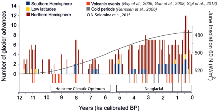
Figure 43. Global glacier advances during the Holocene. Number of areas that display glacier advances for every century during the Holocene. World glaciers were distributed between 17 geographical areas. 12 belonging to the Northern Hemisphere are represented in brown, 4 from the Southern Hemisphere in blue, and one for the Low Latitudes in yellow. For a geographical representation of the glaciers included in each area see Solomina et al., 2015, figure 1. Orange and grey downward bars represent significant volcanic and cold events respectively according to the references indicated. Grey curve is the June insolation at 60°N (inverted scale). The Neoglacial period is characterized by generalized glacier advances that take place coinciding with the decrease in Northern Hemisphere solar forcing. Source: Courtesy of Olga Solomina.
Cooling events during the HCO, like the 8.2 kyr event, were followed by a complete recovery of temperatures and globally glaciers reached their minimum Holocene extent in most areas between 6000-5500 years BP. However there is evidence that the world did not completely recover from the cooling events that took place between 5600 and 5100 BP, initiating the Neoglaciation. This Mid-Holocene climate reversal has been recorded globally in multiple proxies both as a decrease in temperatures and as hydrological changes (Magny & Haas, 2004; Thompson et al., 2006). While the entire sixth millennium BP had a very challenging climate compared to previous millennia, the cooling event that took place 5.2 kyr BP was particularly abrupt (figure 44, Thompson et al., 2006). Due to the contemporary change of climate regime and global temperatures, some regions became cooler and drier, while others became cooler and wetter, leading to a rapid global glacier advance that buried organic remains, like the Quelccaya Glacier plant (Distichia muscoides, Peru), the South-Cascade Glacier rooted tree-trunk (Washington State) and the Ötztal Alps ice-man, that have remained continuously frozen until the present global warming (Thompson et al., 2006).
Figure 44. Evidence for an abrupt global cold and arid event at 5.2 kyr BP. High and low latitude locations of proxy evidence for abrupt climate change ~ 5,200 yr ago. Evidence for abrupt cooling (blue), aridity (red), flooding (green) and high wind (purple). South-Cascade Glacier rooted tree-trunk (Washington State); remains and artifacts in the Little Salt Spring (Florida); Cariaco Basin metal concentration (Fe, Ti) in ODP site 1002; Quelccaya Glacier ice-buried wetland plant Distichia muscoides (Juncaceae), dated at 5,138 ± 45 yr B.P.; bog pollen records of rapid and drastic vegetation changes in Isla Santa Inés (Chile); eolian soil record from Hólmsá (Iceland); North Atlantic benthic core in ODP site 980; dendrochronological records from Irish and Lancashire oaks with some of their narrowest rings during the 3,195 BC decade; Ötzi, the ice-man from South-Tyrol; core S53 palynological record from Burullus Lagoon (Nile Delta); Soreq Cave (Israel) speleothem; Mauritanian coast core 658C; Kilimanjaro ice-core record; Awafi dry lake sediments in SE Arabia; Lake Mirabad sediment in the Zagros Mountains (Iran); Lunkaransar dry lake sediments in NW India; sedimentary section along the Hongshui River, in the southern Tengger Desert, NW China. From multiple sources, some referenced in L.G. Thompson et al. 2006. PNAS 103, 10536–10543.
Coincident with the abrupt cooling and hydrological changes of ~ 5,200 yr BP, archaeological studies support a general pattern of abandoned Neolithic human settlements in several areas, including the Andes and the entire Eastern Mediterranean, indicating a widespread climatic crisis that marks the transition from the Chalcolithic to the early Bronze Age (Weninger et al., 2009).
Holocene climate variability
The Last Glacial Maximum and the HCO constitute two extreme metastable states, separated by only 10,000 years, that correspond to essentially the same amount of incoming energy from the Sun. The main difference between both states is in the redistribution and minimal or maximal exploitation of that energy by the planet. This is due to the orbital configuration, tectonic disposition, ice and cloud albedo, oceanic-atmosphere response and biological feedback. Since they constitute dramatically different climatic states, the nature of abrupt climatic changes is also different in the two states. Glacial variability comes mainly in the form of warming episodes (Dansgaard-Oeschger events; figure 45) while interglacial variability comes from cooling episodes (Bond events; figure 45). There are no global warming abrupt changes in the Holocene once the thermal maximum is reached, just cooling events followed by recovery.
The other major salient characteristic of the Holocene abrupt climatic changes compared to glacial abrupt changes is their much smaller amplitude (figure 45). It has become a lot more difficult to identify these changes because their signal is much lower and more difficult to separate from the noise of small high frequency climatic variability. This has created much confusion about the nature and causes of Holocene abrupt climatic changes and has given many the false impression that the Holocene is characterized by long periods of climate stability. Nothing is further from the truth. The Holocene is a period of almost constant climate change with climatic stability being the exception.
Figure 45. Nature of climatic oscillations during the Ice Age. Oscillations during an interglacial are smaller and are cooler (Bond) events, and oscillations become larger the colder temperatures become. During the glacial period oscillations are very large and are of a warming nature (Dansgaard-Oeschger events). The black line represents the obliquity cycle. The asterisk marks the current position, where we are very worried that the present warming is the ‘largest in thousands of years’ instead of being worried that the next cooling will also be bigger than the previous and will probably lead to glacial inception.
In 1968 climatologist J. Roger Bray recognized several major past cooling episodes and attributed them to a solar cycle. “A combination of geophysical, biological and glaciological information supports the idea of a 2,600 year solar cycle” (J.R. Bray. 1968. Glaciation and Solar Activity since the Fifth Century BC and the Solar Cycle. Nature 220, 672-674). This solar cycle, slightly shorter than he calculated, is now known as the Hallstatt cycle while, in justice, it should be named the Bray cycle. Since Bray’s report, other researchers have confirmed the reoccurrence of cooler climates with a periodicity of about 2400 – 2600 years by different techniques, glacial moraines, temperature-sensitive tree rings widths, and δ18O isotope and chemical analysis of sea salts and dust in ice cores (O’Brien et al., 1995). Most researchers also ascribe a solar origin to this climatic cycle, since the cooling periods coincide with periods of high Δ14C formation, which is associated with low solar activity.
By looking at proxy temperature reconstructions and at major global glacier advances, and other climate proxies, it is easy to recognize the major abrupt cooling changes of the Holocene. Roger Bray identified cooling episodes at 0.3, 2.8, 5.5, 8.2 and 10.2 kyr BP over 45 years ago (figure 46). These episodes give us an average spacing of ~ 2400 years and, at the same time, they define the major climatic states of the Holocene.
Figure 46. Northern Hemisphere paleoclimate records showing main Holocene abrupt climate change events. (A) Greenland GISP2 ice-core δ18O. (B) Western Mediterranean (Iberian Margin) core MD95-2043, sea surface temperature (SST) C37 alkenones. (C) Eastern Mediterranean core LC21 (SST) fauna. (D) North Atlantic Bond series of drift-ice stacked petrologic tracers. (E) Romania (Steregoiu), mean annual temperature of the coldest month. (F) Gaussian smoothed (200 yr) GISP2 potassium (non-sea salt) ion proxy for the Siberian High pressure system. (G) High resolution GISP2 potassium (non-sea salt). Notice that all Holocene abrupt climate changes are cooling events. Source: B. Weninger et al. 2009. Documenta Praehistorica Vol. 36, pp. 7-59.
The Bray cycle delimits five periods that roughly correspond to the Blytt-Sernander sequence. Vegetation changes suggest that they constitute distinctive climatic states established by insolation conditions from the obliquity and precession cycles (figure 47). Every abrupt cooling from the Bray cycle would constitute a tipping point in the gradual insolation changes and the world would settle to a different climatic state after recovering. We have just started a sixth period with the proposed name of Anthropocene, that should last around 2,200 years, until about 4,200 C.E. Every one of the last five periods (since 10.2 kyr ago) started with global warming as a recovery from the depressed temperatures of the cooling oscillations that separate the periods.
Figure 47. Major periods of the Holocene set by obliquity and a ~2400 year Bray cycle. Black curve, global temperature reconstruction by Marcott et al., 2013, from 73 proxies averaged by differencing and with the original published dates. Temperature anomaly rescaled as in figure 37. Purple curve, Earth’s axis obliquity cycle. Blue boxes, major periods of regional and global glacier advances as in Mayewski et al., 2004 and references within. Red curve, Bond et al., 2001 ice-rafted debris stack (inverted) from four North Atlantic sediment cores. Grey bars, cooling oscillations part of the ~2400 year Bray cycle. Pink bars, the 8.2 kyr cooling event proposed to be due to the outburst of pro-glacial Lake Agassiz and the 4.2 kyr arid-cold event. Grey arches on top, a regular 2475 year periodic marker.
Bond events
In addition to the major cooling events of the Bray cycle, other cooling events have taken place during the Holocene, and they have been seen in numerous proxies, but particularly in the Bond series of events. The amount of detrital petrological tracers transported by icebergs and deposited in the ice-rafted debris belt (an Atlantic region between 40-50° N) greatly increases during episodes of southward and eastward advection of cold surface waters and drift ice from the Nordic and Labrador seas (Bond et al., 2001; figure 48 A). This sensitive proxy has registered every cold episode of the Holocene, with a resolution of 50 years.
Figure 48. Bond events constitute a record of cold events during the Holocene. (A) Map of North Atlantic coring sites. Bond events represent periods of increased deposition of petrological tracers by drift ice at the core locations (black dots) within the ice-rafted debris belt (IRD, yellow box). They are interpreted as periods of cooler, ice-bearing surface waters displaced eastward from the Labrador Sea and southward from the Nordic Seas. (B) The Holocene record of iceberg activity (black curve) is a stack of the four cores showing the combined detrended record of hematite-stained grains, detrital carbonate, and Icelandic volcanic glass. The last drift-ice period corresponds to the Little Ice Age, and other known climatic periods of the past can be correlated to this record. The numbering of enhanced drift-ice periods represents the unsuccessful attempt by Gerard Bond to correlate the now called Bond events with the ~ 1500 year Dansgaard-Oeschger stadial cycle, also reflected in ice-rafted debris records. Source: G. Bond et al., 2001 Science 294, 2130-2136. The Bond cycle is a composite of different periodicities. The early Holocene period clearly displays 1,000 year periodicity as shown by a Gaussian filter applied on the series (green curve). A 1,500 year periodicity is only present from 6,000 yr BP (red curve). The 1,500 year fit is problematic as some peaks appear to follow the 1,000 year periodicity. Source: M. Debret et al., 2007. Clim. Past Discuss., 3, 679–692.
Gerard Bond attempted to fit the periods of increased drift-ice that he identified during the Holocene into a single cycle related to the Dansgaard-Oeschger cycle, by making two unwarranted assumptions: That every period of cooling responded to the same cause, and that some well-resolved peaks separated by several centuries to a millennium could correspond to a single cold event. The evidence, however, shows that the HCO displays a millennial periodicity in Bond events, with single isolated peaks separated by ~ 1000 years, while the Neoglacial shows a more complex picture with multiple peaks not so well resolved and a more irregular spacing. Debret et al. (2007), adjust the Bond record of Holocene cold events to a 1,000 year periodicity between 12 and 7 kyr BP and to a 1,500 year periodicity for the last 6,000 years (figure 48 B). It is clear that the Bond record mixed periodicity reflects the climatic shift that took place at the MHT from mainly solar forcing to a mixed solar and oceanic forcing (figure 41), and therefore it can be concluded that the first assumption of Gerard Bond is incorrect: different peaks represent cooling from different causes, and thus a Bond cycle does not exist in the Holocene. We must reject also his second assumption and treat every peak as a different cooling event and try to identify the cause that originated it. We must move from a Bond series of 8 events (plus number zero) in 12,000 years (one event every 1500 years), to a series of at least 15 cold events with a mixture of periodicities during the Holocene.
The lows of the ~ 2400 year Bray cycle, the main climatic cycle during the Holocene, correspond to Bond events 7, 5a, 4a, 2a, and 0. These events not only show a corresponding age and correct periodicity, but they also constitute the highest petrological tracer peaks for each 2400 year period, suggesting that they were the strongest cooling periods at each time, as glaciological, biological and geophysical evidence also supports.
Holocene millennial cycles
As we have seen in part I and II of the series, low frequency-high amplitude climate change does not take place in a chaotic manner, but mainly through cycles, quasicycles, and oscillations that respond to periodic changes in the forcings that act over the climate system. Figure 49 (adapted from Maslin et al., 2001) shows that these climatic periodicities cover the full spectrum of climate variation, and that, in general, the longer periodicities produce larger variations in climate. Thus Holocene climate change is dominated by periodic variability in the millennial band (grey band, figure 49).
Figure 49. Climate cycles and periodicities dominate climate change at all temporal scales. Spectrum of climate variance showing the better studied climatic cycles and their proposed forcings, although some are not widely accepted. Cycles, quasicycles, and periodic oscillations are found over the entire temporal range, indicating they are a salient property of climatic variability. As a general rule, the lower the frequency, the more intense the climatic variance produced. The 150 Myr Ice Age cycle has produced four Ice Ages in the last 450 million years. It is proposed to be caused by the crossing of the galactic arms by the Solar system. The 32 Myr cycle has produced two cycles during the Cenozoic era, the first ending in the glaciation of Antarctica and the second in the current Quaternary Ice Age. It is proposed to be caused by the vertical displacement of the Solar system with respect to the galactic plane. The orbital or Milankovitch cycles are the best studied, and between them and the Lunar nodal regression cycle of 18.6 years lies the orbital gap, where no astronomical cycle is known to affect climate. Our knowledge of this range is very insufficient, despite millennial climate cycles (grey band) determining most of Holocene climatic variability. Short term climate variability is dominated by the El Niño-Southern Oscillation. Adapted from: M. Maslin, et al. 2001. Geophysical Monograph Series 126. pp. 9-52.
Within the paleo-climatological scientific community there is widespread acceptance of millennial cycles during the Holocene because their effects are observed in most climatic proxies, and there is ample agreement over certain periodicities that come out of frequency analysis and are in phase from multiple proxies at different locations. Instrumental-era climatologists and astrophysicists are however very skeptical of such periodicities because they have not collected evidence about these long cycles in the short time of modern instrument observations, and we lack a proper understanding of the mechanisms that generate the periodicity and produce the climatic effect. Similar objections were made to Alfred Wegener’s continental drift theory that despite solid evidence from geography, geology, paleontology, and biology, was shunned until the development of plate tectonics theory could explain how continents drifted.
A further complication arises because some climate periodicities do not show the behavior of proper cycles and present gaps when the signal cannot be detected in the data. We already observed that problem when reviewing the Dansgaard-Oeschger cycle, where the oscillations depend on a set of conditions in sea-level, temperatures, and obliquity, to become perceptible. Wavelet analysis of millennial climate cycles during the Holocene shows periods when one or more of the currently operable cycles do not show up in the data. As we do not have a proper knowledge of the mechanisms of these cycles, we do not have an explanation for this behavior. And we also have to consider the awkward nature of most climate proxy data (Witt & Schumann, 2005), which is affected by random and systemic errors causing uncertainties along the age axis that grow worse as we go back in time. This data is often unevenly sampled and has increasing compression with growing age, causing a reduction in data density in the older portion of the data. It also suffers from different noise intensity for different paleoclimatic periods and is affected by changing sampling rates. Quite often this awkward nature of paleoclimatic proxy data is not properly accounted for when performing standard time series analyses, which were developed for evenly sampled and stationary time series over a well-defined time axis.
Despite these problems, three relatively well established millennial-scale climatic periodicities can be described based on evidence. They are the already mentioned ~ 2400 year Bray solar variability cycle, a ~ 1500 year oceanic cycle that might be related to the D-O cycle of glacial periods, and the ~ 1000 year Eddy solar variability cycle. As mentioned above, Holocene cycles display abrupt cooling at their lows, creating the conditions for enhanced iceberg activity in the North Atlantic that produces Bond ice-rafting events. As the three cycles have different periodicities, sometimes the lows of two cycles are so close together in time as to make it difficult to resolve them. This is the case in the Little Ice Age, when the lows of all three cycles took place in close succession, contributing to make this the coldest period in the Holocene, bringing it to the brink of triggering a glacial period. After each abrupt cooling of the lows of these three cycles comes a warming recovery, that was a complete recovery during the HCO, but only partially complete during the Neoglacial. The global warming that has taken place during the last 350 years cannot be separated from the previous cooling without losing part of its context. As already indicated in figure 46, each period of warming during the descent to the next glacial stage should be more intense than the previous ones, as climatic variability increases outside the warm conditions of an interglacial climatic optimum.
Conclusions
6) The Neoglacial has been a period of progressive cooling, increasing aridity, and advancing glaciers, delimited by the 5.2 kyr event at its beginning and the Little Ice Age at its end.
7) Holocene climate variability is characterized by periodic cooling events of reduced amplitude compared to glacial climate variability. The main climatic cycle of ~ 2400 years delimits five periods of consistent climatic conditions identified over a century ago in the Blytt-Sernander sequence, separated by abrupt climatic changes.
8) Additional Holocene abrupt climatic variability is reflected in Bond peaks of increased drift ice in the North Atlantic. Abrupt Holocene variability responds mainly to periodicities in the millennial time frame. Abrupt Holocene changes have all been of a cooling nature, followed by global warming.
9) Bond events display a mixture of periodicities that respond to different forcings, thus a Bond cycle does not exist in the Holocene.
Acknowledgements
I thank Andy May for reading the manuscript and improving its English.
References [bibliography ]
Moderation note: As with all guest posts, please keep your comments civil and relevant.Filed under: Attribution, Data and observations