by Javier
First in a two part series on Holocene climate variability.
Summary: Holocene climate is characterized by two initial millennia of fast warming followed by four millennia of higher temperatures and humidity, and a progressively accelerating cooling and drying for the past six millennia. These changes are driven by variations in the obliquity of the Earth’s axis. The four millennia of warmer temperatures are called the Holocene Climatic Optimum which was 1-2°C warmer than the Little Ice Age. This climatic optimum was when global glaciers reached their minimum extent. The Mid-Holocene Transition, caused by orbital variations, brought a change in climatic mode, from solar to oceanic dominated forcing. This transition displaced the climatic equator, ended the African Humid Period and increased El Niño activity.
Introduction
A review of abrupt climate changes of the recent past provides a frame of reference for current global warming. The glacial cycle was reviewed in the first article in the series. The second article focused on the Dansgaard-Oeschger cycle that characterizes glacial periods. In this article I review the general features of Holocene climate, limiting it to the period ending in the 0 yr BP (year zero before present), that is established by geologists and paleoclimatologists as 1950.
As we saw in the previous article, botanists studying peat stratigraphy were among the first to notice, in the late 19th and early 20th century, abrupt climate changes reflected in peat layers. These sudden transitions were later confirmed by changes in sediment pollen composition. Scandinavian palynologists established the Blytt-Sernander sequence which divided the Holocene into five periods. They used the terms Boreal for drier, and Atlantic for wetter (figure 33).
Figure 33. Pollen diagram at Roskilde Fjord. An example of the Blytt-Sernander climatic zones established with the traditional pollen indicators, with the distinct elm-fall at the Atlantic/Sub-Boreal transition, and the rise of beech at the Sub-Boreal/Sub-Atlantic transition. Period dates might change at different locations. Source: N. Schrøder et al. 2004. J. Transdiscip. Environ. Stud. 3 1-27.
The Blytt-Sernander sequence fell out of fashion in the 1970s when new techniques allowed a more quantitative reconstruction of past climates. However, it captures the essence of Holocene climate as four periods of roughly 2500 years each. Every period shows a characteristic vegetation pattern indicative of stable climatic conditions, separated from other periods by rapid vegetation changes suggestive of abrupt climate changes. The dates and conditions generally accepted (Encyclopedia of Environmental Change) are:
– Pre-Boreal, 11,500 – 10,500 yr BP. Cool and sub-arctic.
– Boreal, 10,500 – 7,800 yr BP. Warm and dry.
– Atlantic, 7,800 – 5,700 yr BP. Warmest and wet.
– Sub-Boreal, 5,700 – 2,600 yr BP. Warm and dry.
– Sub-Atlantic, 2,600 – 0 yr BP. Cool and wet.
The transition from Sub-Boreal to Sub-Atlantic took place at the end of the Bronze Age. Rutger Sernander proposed that this climatic change was abrupt, even a catastrophe that he identified with the Fimbulwinter of the Sagas. At the time other scientists believed in a more gradual climatic change, but recent studies on the 2.8 kyr abrupt cooling event (Kobashi et al., 2013) agree with Sernander.
Another classification divides the Holocene climatically into two periods: the Holocene Climatic Optimum (HCO, also known as Hypsithermal or Holocene Thermal Maximum), between 9,000 and 5,500 yr BP (although some authors only consider it from 7,500 yr BP after the 8.2 kyr event), and the Neoglacial period, between 5,000 and 100 yr BP, separated by the Mid-Holocene Transition (MHT) that roughly coincides with the start of the Bronze Age.
Finally other authors divide the Holocene in three periods. The Early Holocene, up to the 8.2 Kyr event, the Middle Holocene, between the 8.2 and the 4.2 Kyr events, and the Late Holocene since the 4.2 Kyr event. Although this is currently the most popular subdivision, in my opinion, it fails to properly capture the climatic trends of the Holocene.
Holocene general climate trend
Broadly speaking the Holocene had an abrupt start at 11,700 yr BP, after the Younger Dryas cold relapse, and reached maximal temperatures in about 2,000 years. Since about 9,500 yr BP, a time that coincides with maximal obliquity of the Earth axis, the climate of the Holocene stopped warming and a few thousand years later started a progressive cooling.
By far the main factor driving Holocene climatic change are the insolation changes due to the orbital variations of the Earth (figure 34). These changes are of two types that produce two different effects not always properly differentiated by Holocene climate researchers. Changes due to precession (modulated by eccentricity) have the effect of redistributing insolation between the different seasons of the year by latitude. The 23,000-year precession cycle determines the direction each hemisphere is pointing towards at perihelion and aphelion, and thus the amount of insolation received by each hemisphere at any point of the orbit. Insolation changes due to precession are represented in figure 34 with three month insolation curves for a North and South latitude, relative to present values. These changes increase or decrease seasonality or the difference between summer and winter. So, Northern Hemisphere seasonality was minimal at the Last Glacial Maximum, and maximal at the start of the Holocene, 10,500 yr BP, and will become minimal again in a thousand years.
Precession changes do not alter the annual amount of insolation at any latitude, since whatever insolation they take from one month at a particular location, they give back in another month within the same year. Precession changes are also asymmetrical, as their effect is opposite in each hemisphere, so the Northern Hemisphere summer (June-August, N-JJA thick red line in figure 34) has become progressively cooler during most of the Holocene, while Southern Hemisphere summer (December-February, S-DJF thick blue line in figure 34) has become progressively warmer during most of the Holocene. Precession changes are responsible for sea surface temperature (SST) patterns, and thus oceanic currents. North-South differences set the position of the ITCZ (Intertropical Convergence Zone or the climatic equator). Therefore they are responsible for the African Humid Period, monsoon patterns and the important Mid-Holocene Transition (MHT), that changed the climate mode of the Holocene globally.
Figure 34. Insolation changes due to orbital variations of the Earth. The insolation changes for the last 40,000 years are represented. Black temperature proxy curve represents δ18O isotope changes from NGRIP Greenland ice core (without scale). The insolation curves are presented as the insolation anomaly for summer, winter, spring, and fall. N (red) or S (blue) are the Northern or Southern Hemisphere and the three letters are the month initials. Northern and southern summer insolation represented with thick curves. Background color represents changes in annual insolation by latitude and time due to changes in the Earth’s axial tilt (obliquity), shown in a colored scale. This figure essentially shows how global temperature changes respond mainly to persistent changes in insolation caused by changes in obliquity that are symmetrical for both poles. Changes in seasonality insolation caused by the precession cycle (modified by eccentricity) are asymmetric and less important for the global response, although they cause profound changes in regional climatic differences. The Holocene Climatic Optimum corresponds to high insolation surplus in polar latitudes (red area), while Neoglacial conditions represent the first 5,000 years of a 10,000 year drop into a high glacial insolation deficit in polar latitudes (blue area). Sources: Insolation curves: P.J. Polissar et al. 2013. PNAS Vol. 110 No. 36 pp. 14551–14556. NGRIP δ18O isotope curve: NGRIP members. 2004. Nature, 431, 147-151. Background color: Steve Carson. The science of Doom.
Changes due to obliquity have the effect of redistributing insolation between different latitudes following an obliquity cycle of 41,000 years. When obliquity was maximal 9,500 years ago, both poles received more insolation due to obliquity, while the tropics received less. Obliquity also affects seasonality, at maximal axial tilt, there is an increased difference between summer and winter at high latitudes. But unlike precession changes, obliquity alters the amount of annual insolation at different latitudes in a 41,000 year cycle. This is represented by the background color of figure 34, that shows how the polar regions received increasing insolation from 30,000 yr BP to 9,500 yr BP. Since then, and for the next 11,500 years, the poles will be receiving decreasing insolation. Unlike precessional insolation changes, obliquity changes are symmetrical. Although the annual insolation change is not too large, it accumulates over tens of thousands of years and the total change is staggering, creating a huge insolation deficit or surplus. This changes the equator-to-pole temperature gradient, and is largely responsible for entering and exiting glacial periods (Tzedakis et al., 2017) and for the general evolution of global temperatures and climate during the Holocene. Obliquity changes contribute to the lack of warming of Antarctica during the Holocene, despite increasing Southern Hemisphere summer insolation. Ultimately obliquity changes will be responsible for the glacial inception that will put an end to the Holocene interglacial in the distant future.
In the Holocene, the precession cycle and the obliquity cycle are almost aligned so that maximal obliquity and maximal northern summer insolation are almost coincident at the beginning of the interglacial about 10,000 years ago. See in figure 34 how the thick red curve representing northern summer insolation reaches maximal values 10 kyr BP, almost coinciding with the center of the background polar red color, representing highest warming from maximal obliquity about 9.5 kyr BP. However this has an interesting consequence. 19,000 years ago obliquity was the same as it is now (only increasing), and the precession cycle was at the same position as it is now (same 65 °N summer insolation; figure 34). The Earth was receiving the same energy from the Sun, and the orbital configuration was distributing it over the planet in the same way during the Last Glacial Maximum as today. Why is the climate so different for the same energy input?
The answer is the huge thermal inertia of the planet due mainly to its water content. 21,000 years ago the increasing obliquity had been adding energy to the poles for 10,000 years, reducing the insolation latitudinal gradient (Raymo & Nisancioglu, 2003), and adding energy to the summers (Huybers, 2006; Tzedakis et al., 2017), and was on its way to overcome the huge cold inertia with the help of precession changes that were about to take place. In the present, decreasing obliquity has been taking energy from the poles for 10,000 years, increasing the insolation latitudinal gradient that favors energy loss and increased polar precipitation, and reducing energy during summers. These changes will also overcome the huge warm inertia even against precession changes, but will do so progressively for many thousands of years. A comparison between temperatures and obliquity over the past 800,000 years shows that while variable, the thermal inertia of the planet delays the temperature response to obliquity changes by an average of 6,500 years (figure 35).
Figure 35. Temperature changes due to axial tilt changes. Black curve, temperature anomaly in degrees centigrade at EPICA Dome C ice core for the past 800,000 years, lagged 6,500 years. Grey curve changes in obliquity of the planetary axis in degrees. The drop of obliquity always terminates interglacials. Sources: EPICA Dome C data: Jouzel, J., et al. 2007 Science, 317, 5839, 793-797. Astronomical data: Laskar, J., et al. 2004 A&A 428, 261-285.
On a multi-millennial scale, global average temperatures follow mainly the 41,000 year obliquity cycle with a lag of several thousand years. Holocene temperatures are no exception, and a few thousand years after the peak in obliquity (9,500 years ago), temperatures started to decline. This general pattern of Holocene temperatures was already known by the late 1950’s from a variety of proxy records from different disciplines (Lamb, 1977; figure 36 A). Greenland ice cores confirmed this pattern, when corrected for uplift (Vinther et al., 2009), and greatly improved the dating of temperature changes (figure 36 B).
Figure 36. Holocene temperature profile. A. Summer (July-August) Central England temperature reconstruction from multiple proxies and sources by H. H. Lamb.Crosses represent dating and temperature uncertainty. Black dots are centennial averages. Red dot is 1900-1965 average. Source: Lamb, H.H. 1977. Climate: Present, past and future. Volume 2. B. Greenland temperature reconstruction based on an average of uplift corrected δ18O isotopic data from Agassiz and Renland ice cores. This average has been corrected for changes in the δ18O of seawater and calibrated to borehole temperature records. Some historical periods are indicated. Source: B. Vinther et al., 2009.
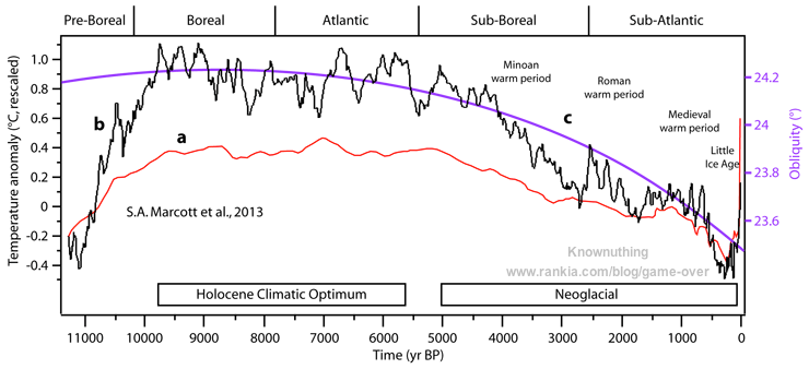
There is only one Holocene global average temperature reconstruction available (Marcott et al., 2013; figure 37 a). To correct some of the problems it presents, I use this reconstruction averaged by differencing (explained here), without any smoothing, and with the original published dates for the proxies. I have also rescaled the temperature changes to make them congruent with the vast literature and consilience of evidence from different fields that indicates that the Holocene Climatic Optimum was on average between 1 and 2 °C warmer than the Little Ice Age (figure 37 b). This rescaling is discussed below. The resulting temperature curve is extraordinarily similar to H. Lamb regional reconstruction from the 1970s (figure 36 A), with significant temperature drops at 5.5, 3, and 0.5 kyr BP.
Figure 37. Holocene global temperature change reconstruction. a. Red curve, global average temperature reconstruction from Marcott et al., 2013, figure 1. The averaging method does not correct for proxy drop out which produces an artificially enhanced terminal spike, while the Monte Carlo smoothing eliminates most variability information. b. Black curve, global average temperature reconstruction from Marcott et al., 2013, using proxy published dates, and differencing average. Temperature anomaly was rescaled to match biological, glaciological, and marine sedimentary evidence, indicating the Holocene Climate Optimum was about 1.2°C warmer than LIA. c. Purple curve, Earth’s axis obliquity is shown to display a similar trend to Holocene temperatures. Source: Marcott et al., 2013.
The controversial role of greenhouse gases during the Holocene
What role, if any, have greenhouse gases (GHG) played in Holocene climate change? Available data indicates that despite significant changes in GHG concentration in the atmosphere during the period of 10,000 to 600 yr BP, their contribution to temperature changes cannot have been important.
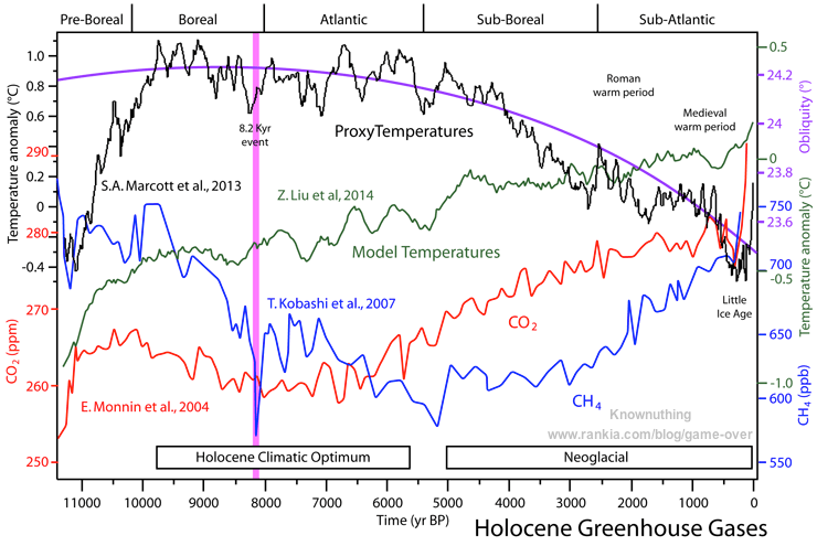
According to Monnin et al. (2004), CO2 concentrations measured in Antarctic ice cores decreased from 267 to 258 ppm between 10,000 and 6,800 yr BP, and afterwards increased more or less linearly to 283 ppm by 600 yr BP, just prior to the LIA (figure 38). This increase of 25 ppm represents about 10% of a doubling. Consider the period from the Last Glacial Maximum (20 kyr BP) to the HCO when atmospheric CO2 increased from 70 ppm or 36% of a doubling. We can see that the Holocene CO2 increase constitutes 27% of the CO2 increase from the coldest point of the last glacial period to the warmest point of the present interglacial. Almost a third of the glacial-interglacial span cannot be considered insignificant for the increase in CO2 that took place between 6,800 and 600 yr BP. If CO2 is as potent warming agent as purported in some theories and models, one should expect some warming coming out of this CO2 increase, especially because from 5,000 yr BP it was accompanied by an increase in atmospheric CH4 concentrations (Kobashi et al., 2007; figure 38). But instead of an increase in temperatures, what we find is a progressive decrease from the HCO to the LIA driven by changes in insolation.
Figure 38. Temperature and greenhouse gases changes during the Holocene. Black curve, global temperature reconstruction by Marcott et al., 2013, as in figure 37. Purple curve, Earth’s axis obliquity cycle. Red curve, CO2 levels as measured in Epica Dome C (Antarctica) ice core, reported in Monnin et al., 2004. Blue curve, methane levels as measured in GISP2 (Greenland) ice core from Kobashi et al., 2007. Notice the great effect of the 8.2 kyr event on methane concentrations. Green curve, simulated global temperatures from an ensemble of three models (CCSM3, FAMOUS, and LOVECLIM) from Liu et al., 2014, show the inability of general climate models to replicate the Holocene general temperature downward trend. Pink bar, 8.2 kyr BP climatic event. Major Holocene climatic periods are indicated.
Climate models adjusted to explain present global warming do not reproduce the Holocene climate. The mean temperatures of an ensemble of three models (CCSM3, FAMOUS, and LOVECLIM; Liu et al., 2014; figure 38) show a constant increase in temperatures during the entire Holocene, driven by the increase in GHG. This disagreement between models and data-derived reconstructions of Holocene climate has been termed by the authors the Holocene temperature conundrum (Liu et al., 2014).
Climate modelers should take the opportunity to adjust their models to Holocene conditions. It is clear that the main driver of Holocene climate has been changes in insolation due to orbital variation. Changes in GHG concentrations appear to have had only a minor effect.
The Holocene Climatic Optimum
The issue of Holocene temperatures has become controversial. While the Holocene Hypsithermal or Climatic Optimum (HCO, ~ 9800-5700 BP) is well characterized in the Northern Hemisphere as 1-5°C warmer than the bottom of the LIA depending on latitude, much less information exists regarding the tropical and Southern areas. Marcott et al. (2013), take the view that, globally, the HCO was 0.7°C warmer than the bottom of the LIA. Such low temperature variability for the Holocene rests on tropical warming of 0.4°C during the HCO, and Southern area HCO cooling of 0.4°C.
At the core of the issue is the question: are current temperatures outside the registered bounds for Holocene temperatures? The cryosphere clearly shows that glaciers all over the world were significantly more reduced during the HCO than at present (Koch et al., 2014). The biosphere generally agrees since the extension of species such as the water chestnut and the pond turtle were then north of their present European climatic limits and the treeline has not reached its HCO maximum latitude or altitude in Sweden (Kullman, 2001), Canada (Pisaric et al., 2003), Russia (MacDonald et al., 2000), the Alps (Tinner et al., 1996), or Colombia (Thouret et al., 1996). The marine biosphere agrees as current levels of coccolithophores in the tropical oceans are lower than during the HCO (Werne et al., 2000), which is another indication that the oceans are not as warm as then.
In contrast to Marcott et al. (2013), the non-tropical Southern Hemisphere post HCO Neoglacial cooling is well documented in the many glaciers from the Southern Andes and New Zealand reviewed by Porter (2000). Their data demonstrates that Southern Hemisphere glaciers were smaller during the HCO, and that the early Neoglacial advance began between 5400-4900 BP. In southern Africa, Holmgren et al. (2003) have shown persistent Holocene cooling since 10,000 yr BP. In Antarctica Masson et al. (2000), identify an early Holocene optimum at 11,500-9,000 BP followed by a second optimum at 7,000-5,000 BP. Shevenell et al. (2011), show that the Southern Ocean has cooled by 2-4°C at several locations in the past 10-12 kyr. The Holocene cooling of just 0.4°C proposed by Marcott et al. (2013) for the Southern 30-90°S region appears to be an underestimation. At Southern latitudes, the HCO cannot be explained by precessional summer insolation changes, and large-scale reorganization of latitudinal heat transport has instead been invoked. Decreasing obliquity should also be considered a cause.
However, it is in the tropical areas where Marcott et al. (2013) becomes more controversial. The fossil coral Sr/Ca record at the Great Barrier Reef, Australia, shows that the mean SST ~ 5350 BP was 1.2°C warmer than the mean SST for the early 1990s (Gagan et al., 1998). At the Indo-Pacific Warm Pool, the warmest ocean region in the world, Stott et al. (2004) find that SST has decreased by ~ 0.5°C in the last 10,000 years, a finding confirmed by Rosenthal et al. (2013), who show a decrease of 1.5-2°C for intermediate waters. East African lakes show temperatures peaking toward the end of the HCO, followed by a general decrease of 2-3°C to the LIA (Berke et al., 2012). Tropical glaciers at Peru (Huascarán) and Tanzania (Kilimanjaro) display their highest δ18O values (warmest) at the HCO, followed by a general decline afterwards (Thompson et al., 2006). The position that the tropics have experienced warming since the HCO appear to be based, in large part, on marine alkenone proxies, however many alkenone records are from upwelling areas that have high sedimentation rates, but often display inverted temperature trends. Even worse, they generally do not agree with Mg/Ca proxies. Leduc et al. (2010) attempt to resolve the discrepancy between these two paleo-thermometry methods and note that none of the seven Mg/Ca records available for the East Equatorial Pacific have exhibited monotonous warming during the Holocene. They attribute the discrepancy with the alkenone annual temperature signal, by suggesting that it only captures the winter season and thus responds mainly to changes in insolation during that season. This explanation brings the divergent alkenone records in agreement with the rest of the marine and land tropical records that display a tropical cooling since the HCO. If we estimate this cooling in the 0.5-1°C range it is clear that Marcott et al. (2013) are underestimating global Holocene cooling and therefore HCO global temperatures.
An estimate of ~ 1.2°C global temperature decrease between average HCO temperatures and the bottom of the LIA is therefore consistent with global proxies, glaciological changes, and biological evidence. Model reconstructions (Renssen et al., 2012) also disagree with Marcott et al., 2013 since they show warming in the tropical areas during the HCO with respect to pre-industrial temperatures.
The Mid-Holocene Transition and the end of the African Humid Period
The MHT is a period of time between 6,000 and 4,500 yr BP when a global climatic shift took place at a time of significant human cultural changes that are associated with the transition from the Neolithic to the Bronze Age. The MHT separates the HCO from the Neoglacial, and is characterized by periods of global glacier advance interrupted by periods of partial recovery.
The principal cause of this global climatic shift was the redistribution of solar energy as the northern summer insolation decrease reached its maximum rate. This redistribution of solar energy, due to orbital forcing, produced a progressive southward shift of the Northern Hemisphere summer position of the Intertropical Convergence Zone (ITCZ). This accompanied a pronounced weakening of summer monsoons in Africa and Asia and increased dryness and desertification at around 30°N latitude in South America, Africa and Asia. The associated summertime cooling of the NH, combined with changing latitudinal temperature gradients in the world oceans, likely led to an increase in the amplitude of the El Niño Southern Oscillation (ENSO). The effect of these changes had world wide repercussions in temperature and precipitation patterns (figure 39).
Figure 39. Climate pattern change at the Mid-Holocene Transition. The shift from the Holocene Thermal Maximum to the Neoglacial involved a complete reorganization of the Earth’s climate, mainly directed by the southward migration of the Intertropical Convergence Zone (ITCZ) and the weakening of the African, Indian and Asian summer monsoons Source: H. Wanner & S. Brönnimann, 2012. PAGES news 20, 44-45.
The 23 kyr precession cycle is the main force behind the seasonal changes in the North-South temperature gradient that are so important for the climate in general and the precipitation regime of the ~30°N tropical band. The orbital monsoon hypothesis was first proposed by Kutzbatch (1981) and is supported by current evidence. Rossignol-Strick (1985) demonstrated that the dark organic-rich layers in the Mediterranean sediments, known as sapropels, represent periods of intense African monsoon every 23 kyr, modulated by the precession and eccentricity cycles. These sapropel formation periods also correspond to African Humid Periods, when the African monsoon produces enough precipitation over the Sahara to sustain a savanna type ecosystem. The last such period started about 15 kyr BP, but had a dry interval during the Younger Dryas at 12.5 kyr BP. As the Sahara became covered in vegetation, with large rivers and lakes, and populated by large mammals, it became inhabited by humans (figure 40). The Green Sahara entered a dryness crisis around 5.8 kyr BP and became a desert in just 500 years when the ecosystem collapsed and its human population crashed. Climate refugees from the Sahara greatly increased the population in the Nile valley and shortly after 5500 BP Egyptian society began to grow and advance rapidly towards refined civilization. Extensive use of copper became common during this time (Chalcolithic Period). The process culminated 5100 yr BP with the unification of Egypt under the first pharaoh in one of the first complex civilizations.
Figure 40. The African Humid Period. A. Climate-controlled occupation in the Eastern Sahara during the main phases of the Holocene. Red dots indicate major occupation areas; open dots indicate isolated settlements. During the Last Glacial Maximum and the terminal Pleistocene (20,000 to 12,500 BP), the Saharan desert was void of any settlement outside of the Nile valley. With the abrupt arrival of monsoon rains at 12,500 BP, the desert was replaced by savannah-like environments and became inhabited by prehistoric settlers. After 9,000 BP, human settlements became well established all over the Eastern Sahara, fostering the development of cattle pastoralism. Retreating monsoonal rains caused the onset of desiccation of the Egyptian Sahara at 6,300 BP. Prehistoric populations were forced to the Nile valley. The return of full desert conditions all over Egypt at about 5,500 BP coincided with the initial stages of pharaonic civilization in the Nile valley. Source: R. Kuper & S. Kröpelin. 2006. Science 313, 803-807. B. Dust flux (aridity proxy, red curve, inverted) record from the NW African coast 658C core related to a population proxy (black curve) based in the summed probability distribution of 3287 calibrated 14C ages from 1011 archeological sites between 14,000-2,000 years BP. Dotted lines indicate the concurrent end of the African Humid Period and population collapse. Source: K. Manning & A. Timpson. 2014. Quat. Sci. Rev. 101, 28-35.
Several authors have noticed that the MHT (6,000 to 4,500 yr BP), in addition to a global climatic pattern change, also underwent a significant change in the principal climate forcings. Debret et al. (2009) after studying 15 climate proxies from marine sediments (North Atlantic, West Africa and Antarctic), ice-core records (South America and Antarctica), cave speleothems (Ireland) and lacustrine sediments (Ecuador) by wavelet analysis, concluded that the first part of the Holocene was characterized by frequencies typical of high solar activity at 1000 years and 2500 years. The 2500 year frequency is continuous throughout the Holocene (figure 41 F). Around 5,000 years BP, the Thermohaline Circulation was finally stabilized for the second half of the Holocene (figure 41 D). MHT is a key period in the Holocene since many parameters influencing weather or climate changed abruptly. Sea level stopped increasing (figure 41 E), the flow of meltwater became insignificant, and insolation reached its maximum variation (figure 41 C). The millennial solar cycle disappeared in favor of a cyclical internal (ocean) forcing (figure 41 F).
Figure 41. Bimodal pattern of global climate during the Holocene. Global climate is dominated by a spectral imprint attributed to solar forcing (red bars) during the Holocene Thermal Maximum (HTM), and to oceanic forcing (blue bars) during the Neoglacial. (A) Glacial activity indicated by soil particles content (rAP) in Lake Blanc Huez (Alps) LBH06 core interpreted as a runoff process marker largely due to snowmelt. (B) Total Organic Carbon (TOC) values, anti-correlated to lightness (L*) fluctuations given by spectrophotometry as an indicator of glacial activity. (C) Solar energy. And (D) the North-Atlantic circulation evolution over the Holocene reflected by sea surface temperature (SST) in the North Atlantic. The light gray hatched area represents the Mid-Holocene Transition from one mode to the other. Source: S. Simonneau et al. 2014. Quat. Sci. Rev. 89, 27-43. (E) Sea Level reaches near maximum height at this time. (F) Frequency pattern based on wavelet analysis of a variety of proxies from different locations shows the first half of the Holocene dominated by frequencies attributed to solar forcing (red bars), while the second half of the Holocene sees a decrease in forcing from some solar frequencies and an increase from frequencies attributed to oceanic forcing (blue bars), together with an increase in ENSO forcing (green bar). Source: M. Debret et al. 2009. Quat. Sci. Rev., 28, 2675-2688.
Similar conclusions were reached by Simonneau et al. (2014), studying proglacial lacustrine sediments in the Alps. They show that over the last 9,700 years, the Holocene lake record has a bimodal pattern whose transition is gradual and occurred between 5,400 and 4,700 yr BP. The Early Holocene is characterized by reduced glacial activity due to increasing solar forcing and high summer insolation. After 5,400 yr BP, lacustrine sedimentation is marked by a gradual increase of minerogenic sediments and a reduction in organic content, suggesting a transition to wetter climatic conditions (figure 41 A & B). This climate change is synchronous with the gradual decrease of summer insolation and the gradual reorganization of oceanic and atmospheric circulation, characterizing the beginning of the Neoglacial period.
A bimodal climate pattern was also identified during the Holocene by Moy et al. (2002) in the Laguna Pallcacocha sediment proxy for ENSO activity for the last 12 kyr (figure 42). They found the HCO was dominated by millennial solar forcing and the Neoglacial was dominated by oceanic-atmospheric forcing. These periods were separated by the MHT. ENSO activity was essentially absent during most of the HCO and first becomes statistically significant around 7,000 yr BP, increasing considerably after 5,600 yr BP, and displaying many very strong peaks of activity during the Neoglacial period. Moy et al. also observe that periods of high North Atlantic iceberg activity, indicative of significant cooling (Bond events) tend to occur during periods of low ENSO activity immediately following a period of high ENSO activity. This suggests that some link may exist between the two systems (figure 42; Moy et al., 2002).
Figure 42. Distribution of El Niño Southern Oscillation (ENSO) activity during the Holocene. ENSO activity also displays a bimodal distribution, with low ENSO activity during the HCO and high ENSO activity during the Neoglacial. Cold Bond events, marked by increases in ice-rafted debris (inverted), tend to occur immediately following periods of high ENSO activity, and coincide with periods of low ENSO activity.
From a thermodynamic point of view high ENSO activity transfers great amounts of heat from the ocean sub-surface to the atmosphere, and afterwards a great part of that heat is radiated to space. This constitutes a cooling event from a whole Earth climate system perspective, even if it appears as warming from a lower atmosphere perspective. It is proposed that high ENSO activity is made possible by a high equator-to-pole temperature gradient. During the HCO the temperature gradient was kept low by high polar insolation due to high obliquity. After 7,000 yr BP the decrease in polar insolation and the increase in tropical insolation favored a progressive increase in the gradient, especially during prolonged periods without significant cooling, i.e. immediately preceding a Bond event. The profound cooling from a Bond event would eliminate or greatly reduce ENSO activity by quenching the thermal energy required for an El Niño event. If correct, high ENSO activity would be a sign of a cooling planet.
Conclusions
1) The Holocene is a period of 11,700 years characterized by an intense warming for about 2,000 years and a progressively accelerating cooling for the last 6,000 years, following the changes in obliquity of the Earth’s axis.
2) Fluctuations in greenhouse gases cannot explain Holocene climatic changes and, indeed, their concentration changes run opposite to temperature trends for most of the Holocene.
3) Climate models perform very poorly when trying to reproduce Holocene climate evolution. This is likely due to having too much sensitivity to changes in greenhouse gases and too little sensitivity to insolation and solar variability.
4) The Holocene Climatic Optimum was a more humid period, 1-2°C warmer than the Little Ice Age, during which global glaciers reached their minimum extent.
5) The Mid-Holocene Transition, caused by orbital changes, brought a complete change in climatic mode, with a decrease in solar forcing and an increase in oceanic forcing, displacing the climatic equator and ending the African Humid Period, while increasing ENSO activity.
Acknowledgements
I thank Andy May for reading the manuscript and improving its English.
[Bibliography]
Moderation note: As with all guest posts, keep your comments civil and relevant.
Filed under: Attribution, Data and observations