by Judith Curry
I have been asked to write an Expert Report on climate models.
***SEE UPDATE
UPDATE: A final version of the report is attached [climate-models]. Thanks a ton to all who provided comments in the blog post and via email, I have incorporated many of these suggestions.
No, I can’t tell you the context for this request (at this time, anyways). But the audience is lawyers.
Here are the specific questions I have been asked to respond to:
- What is a Global Climate Model (GCM)?
- What is the reliability of climate models?
- What are the failings of climate models?
- Are GCM’s are a reliable tool for predicting climate change?
I’ve appended my draft Report below. I tried to avoid giving a ‘science lesson’, and focus on what climate models can and can’t do, focusing on policy relevant applications of climate models. I’ve tried write an essay that would be approved by most climate modelers; at the same time, it has to be understandable by lawyers. I would greatly appreciate your feedback on:
- whether you think lawyers will understand this
- whether the arguments I’ve made are the appropriate ones
- whether I’m missing anything
- anything that could be left out (its a bit long).
——–
What is a Global Climate Model (GCM)?
Global climate models (GCMs) simulate the Earth’s climate system, with modules that simulate the atmosphere, ocean, land surface, sea ice and glaciers. The atmospheric module simulates evolution of the winds, temperature, humidity and atmospheric pressure using complex mathematical equations that can only be solved using computers. These equations are based on fundamental physical principles, such as Newton’s Laws of Motion and the First Law of Thermodynamics.
GCMs also include mathematical equations describing the three-dimensional oceanic circulation, how it transports heat, and how the ocean exchanges heat and moisture with the atmosphere. Climate models include a land surface model that describes how vegetation, soil, and snow or ice cover exchange energy and moisture with the atmosphere. GCMs also include models of sea ice and glacier ice.
To solve these equations on a computer, GCMs divide the atmosphere, oceans, and land into a 3-dimensional grid system (see Figure 1). The equations and are then calculated for each cell in the grid repeatedly for successive time steps that march forward in time throughout the simulation period.
Figure 1. Schematic of a global climate model. https://upload.wikimedia.org/wikipedia/commons/thumb/7/73/AtmosphericModelSchematic.png/350px-AtmosphericModelSchematic.png
The number of cells in the grid system determines the model ‘resolution.’ Common resolutions for a GCM include a horizontal resolution of about 100-200 km, a vertical resolution of about 1 km, and a time stepping resolution that is typically about 30 minutes. While GCMs represent processes more realistically at higher resolution, the computing time required to do the calculations increases substantially at higher resolutions. The coarseness of the model resolution is driven by the available computer resources, and tradeoffs between model resolution, model complexity and the length and number of simulations to be conducted.
Because of the relatively coarse spatial and temporal resolutions of the models, there are many important processes that occur on scales that are smaller than the model resolution (such as clouds and rainfall; see inset in Figure 1). These subgrid-scale processes are represented using ‘parameterizations.’ Parameterizations of subgrid-scale processes are simple formulas based on observations or derivations from more detailed process models. These parameterizations are ‘calibrated’ or ‘tuned’ so that the climate models perform adequately when compared with historical observations.
The actual equations used in the GCM computer codes are only approximations of the physical processes that occur in the climate system. While some of these approximations are highly accurate, others are unavoidably crude. This is because the real processes they represent are either poorly understood or too complex to include in the model given the constraints of the computer system. Of the processes that are most important for climate change, parameterizations related to clouds and precipitation remain the most challenging, and are the greatest source of disagreement among different GCMs.
GCMs are used for the following purposes:
- Simulation of present and past climate states to understand planetary energetics and other complex interactions
- Numerical experiments to understand how the climate system works. Sensitivity experiments are used to turn off, constrain or enhance certain physical processes or external forcings (e.g. CO2, volcanoes, solar output) to see how the system responds.
- Understanding the causes of past climate variability and change (e.g. how much of the change can be attributed to human causes such as CO2, versus natural causes such as solar variations, volcanic eruptions, and slow circulations in the ocean).
- Simulation of future climate states, from decades to centuries, e.g. simulations of future climate states under different emissions scenarios.
- Prediction and attribution of the statistics extreme weather events (e.g. heat waves, droughts, hurricanes)
- Projections of future regional climate variations to support decision making related adaptation to climate change
- Guidance for emissions reduction policies
- Projections of future risks of black swan events (e.g. climate surprises)
The specific objectives of a GCM vary with purpose of the simulation. Generally, when simulating the past climate using a GCM, the objective is to correctly simulate the spatial variation of climate conditions in some average sense. When predicting future climate, the aim is not to simulate conditions in the climate system on any particular day, but to simulate conditions over a longer period—typically decades or more—in such a way that the statistics of the simulated climate will match the statistics of the actual future climate.
There are more than 20 climate modeling groups internationally, that contribute climate model simulations to the IPCC Assessment Reports. Further, many of the individual climate modeling groups contribute simulations from multiple different models. Why are there so many different climate models? Is it possible to pick a ‘best’ climate model?
There are literally thousands of different choices made in the construction of a climate model (e.g. resolution, complexity of the submodels, parameterizations). Each different set of choices produces a different model having different sensitivities. Further, different modeling groups have different focal interests, e.g. long paleoclimate simulations, details of ocean circulations, nuances of the interactions between aerosol particles and clouds, the carbon cycle. These different interests focus computational resources on a particular aspect of simulating the climate system, at the expense of others.
Is it possible to select a ‘best’ model? Well, several models generally show a poorer performance overall when compared with observations. However, the best model depends on how you define ‘best’, and no single model is the best at everything. The more germane issue is to assess model’s ‘fitness for purpose’, which is addressed in Sections 2-4.
The reliability of climate models
Because of the complexity of GCMs, the notion of a correct or incorrect model is not well defined. The relevant issue is how well the model reproduces reality and whether the model is fit for its intended purpose.
Statistician George Box famously stated: “All models are wrong but some are useful.” All models are imperfect; we don’t need a perfect model, just one that serves its purpose. Airplanes are designed using models that are inadequate in their ability to simulate turbulent flow. Financial models based upon crude assumptions about human behavior have been used for decades to manage risk. In the decision making process, models are used more or less depending on a variety of factors, one of which is the credibility of the model.
Climate model development has followed a pathway mostly driven by scientific curiosity and computational limitations. GCMs were originally designed as a tool to help understand how the climate system works. GCMs are used by researchers to represent aspects of climate that are extremely difficult to observe, experiment with theories in a new way by enabling hitherto infeasible calculations, understand a complex system of equations that would otherwise be impenetrable, and explore the system to identify unexpected outcomes. As such, GCMs are an important element of climate research.
Why do scientists have confidence in climate models?
Scientists that evaluate climate models, develop physical process parameterizations, and utilize climate model results are convinced (at least to some degree) of the usefulness of climate models for their research. They are convinced because of the model’s relation to theory and physical understanding of the processes involved, consistency of the simulated responses among different models and different model versions, and the ability of the model and model components to simulate historical observations.
The culture of establishing confidence in climate models is illuminated by considering numerical weather prediction models. Roger Pielke Jr. provides an interesting perspective on this in The Climate Fix:
Decision makers, including most of us as individuals, have enough experience with weather forecasts to be able to reliably characterize their uncertainty and make decisions in the context of that uncertainty. In the U.S., the National Weather Service issues millions of forecasts every year. This provides an extremely valuable body of information experience for calibrating forecasts in the context of decisions that depend on them. The remarkable reduction in loss of life from weather events over the past century is due in part to improved predictive capabilities, but just as important has been our ability to use predictions effectively despite their uncertainties.
This same general strategy for developing confidence is being extended to seasonal climate prediction models, which are based on coupled atmosphere/ocean models. However, on seasonal timescales, skill is assessed in terms of monthly- or seasonally-averaged values. Since the same general formulation for the atmosphere and ocean are used for models across the range of time scales, confidence from the weather and seasonal climate forecast models is transferred to the climate models used in century scale simulations. However, caution is needed in this transferal of confidence, since other factors become significant for the longer timescales in climate models, which have less import in weather models.
User confidence in a forecast model depends critically on the evaluation of the forecasts, both using historical data (hindcasts) and actual forecasts. Evaluation of forecasts is feasible for short time horizons (e.g. weather forecasts). Capturing the phenomena in hindcasts and previous forecasts is a necessary, but not sufficient, condition for the model to capture the phenomena in the future.
Why are some scientists concerned about the reliability of climate models?
Uncertainties in GCMs arise from uncertainty in model structure, model parameters and parameterizations, and initial conditions. Uncertainties in parameter values include uncertain constants and other parameters, subgridscale parameterizations (e.g. clouds), and ad hoc modeling to compensate for the absence of neglected factors. Calibration is necessary to address parameters that are unknown or inapplicable at the model resolution, and also in the linking of submodels. As the complexity of a model grows, model calibration becomes unavoidable and an increasingly important issue. A calibration required in one model may not be required in another model that has greater structural adequacy or higher resolution. Continual ad hoc adjustments of the model (calibration) can mask underlying deficiencies in model structural form. However, it should be noted that in a climate model with millions of degrees of freedom (i.e. different variables, grid cells), it is impossible to tune the model to provide a correct 4D solution of many variables at the same time.
Concerns about evaluating climate models has been raised in context of model calibration/tuning practices; see particularly this recent paper by IPCC coauthors Mauritsen et al. on climate model tuning:
“Climate models ability to simulate the 20th century temperature increase with fidelity has become something of a show-stopper as a model unable to reproduce the 20th century would probably not see publication, and as such it has effectively lost its purpose as a model quality measure. Most other observational datasets sooner or later meet the same destiny, at least beyond the first time they are applied for model evaluation. That is not to say that climate models can be readily adapted to fit any dataset, but once aware of the data we will compare with model output and invariably make decisions in the model development on the basis of the results.”
A remarkable article was recently published in Science: “Climate scientists open up their black boxes to scrutiny.”
“Indeed, whether climate scientists like to admit it or not, nearly every model has been calibrated precisely to the 20th century climate records—otherwise it would have ended up in the trash. “It’s fair to say all models have tuned it,” says Isaac Held, a scientist at the Geophysical Fluid Dynamics Laboratory, another prominent modeling center, in Princeton, New Jersey.”
We are now in a situation whereby matching the 20th century historic temperatures is no longer a good metric for determining which models are good or bad. The implication is that models that match 20th century data as a result of model calibration/tuning are of dubious use for determining the causes of 20th century climate variability.
Agreement between model forecasts/hindcasts and data does not imply that the model gets the correct answer for the right reasons. For example, all of the coupled climate models used in the IPCC Fourth Assessment Report reproduce the time series for the 20th century of globally averaged surface temperature anomalies; yet they have different feedbacks and sensitivities and produce markedly different simulations of the 21st century climate. Success in reproducing past states provides only a limited kind of confidence in simulation of future states.
Broader concerns about climate models have been raised by scientists, engineers and modelers from other fields, outside of climate science. These concerns have been raised in guest posts and comments made at my blog Climate Etc. (judithcurry.com) and also the blog Climate Audit (climateaudit.org). These concerns include:
- GCM predictions of the impact of increasing CO2 on climate cannot be rigorously evaluated for order of a century; climate model development timescales are on the order of a few years, with new model versions emerging every few years.
- Insufficient exploration of model & simulation uncertainty
- Impenetrability of the model and formulation process; extremely large number of modeler degrees of freedom in terms of selecting parameters and parameterizations
- Lack of formal model verification & validation that is the norm for engineering and regulatory science
- Circularity in arguments validating climate models against observations, owing to model tuning/calibration.
- Concerns about a fundamental lack of predictability in a complex nonlinear system characterized by spatio-temporal chaos with changing boundary conditions.
What are the failings of climate models?
As they have matured, GCMs are being increasingly used to provide information to policy makers. Climate model simulations are being used as the basis for international climate and energy policy, so it is important to assess the adequacy of climate models for this purpose. In particular, GCM fitness needs to be assessed for:
- Understanding the causes of 20th century climate change
- Simulation of climate states in the 21st century under different emissions scenarios.
An assessment of the fitness for these two purpose of GCMs will be provided at the end of this section and also in section 4. The focus of this section is on two general topics where GCM simulations are inadequate:
- determination of climate sensitivity to increasing CO2, including the fast thermodynamic feedbacks related to clouds and water vapor that amplify the model sensitivity
- the chaotic nature of the climate system and internal climate variability
Climate sensitivity to CO2
Human-caused warming depends not only on the amount of increase in greenhouse gases but also on how ‘sensitive’ the climate is to these increases. Climate sensitivity is defined as the global surface warming that occurs when the concentration of carbon dioxide in the atmosphere doubles. If climate sensitivity is high, then we can expect substantial warming in the coming century as emissions continue to increase. If climate sensitivity is low, then future warming will be substantially lower.
The equilibrium climate sensitivity (ECS) is defined as the change in global mean surface temperature at equilibrium that is caused by a doubling of the atmospheric CO2 concentration. The IPCC AR4 (2007) conclusion on climate sensitivity is stated as:
“The equilibrium climate sensitivity . . . is likely to be in the range 2oC to 4.5oC with a best estimate of about 3oC and is very unlikely to be less than 1.5oC. Values higher than 4.5oC cannot be excluded.”
The IPCC AR5 (2013) conclusion on climate sensitivity is stated as:
“Equilibrium climate sensitivity is likely in the range 1.5°C to 4.5°C (high confidence), extremely unlikely less than 1°C (high confidence), and very unlikely greater than 6°C (medium confidence)”
This likely range of ECS values varies by a factor of 3. Whether or not human caused global warming is dangerous or not depends critically on whether the ECS value is closer to 1.5oC or 4.5oC. Research over the past 3 decades has not narrowed this range of ECS – the 1979 National Academy of Sciences study – the so-called Charney Report – cited a likely range for ECS that was between 1.5 and 4.5oC.
In fact, it seems that uncertainty about values of ECS has been increasing. The bottom of the ‘likely’ range has been lowered from 2 to 1.5oC in the AR5, whereas the AR4 stated that ECS is very unlikely to be less than 1.5oC. It is also significant that the AR5 does not cite a best estimate, whereas the AR4 cites a best estimate of 3oC. The stated reason for not citing a best estimate in the AR5 is the substantial discrepancy between observation-based estimates of ECS (lower), versus estimates from climate models (higher).
Table 1 compares the values of ECS determined by: the IPCC AR4 (2007), the IPCC AR5 (2013), the CMIP5 climate models cited in the IPCC AR5 (2013), the observational analysis of Lewis and Curry (2014) and the update by Lewis (2015) with lower aerosol forcing,
Table 1: Values of equilibrium climate sensitivity (ECS) (oC)
Lewis and Curry (2014) found values of ECS approximately half that determined from the CMIP5 climate models. Using an observation-based energy balance approach, Lewis and Curry’s calculations used the same data (including uncertainties) for changes in greenhouse gases, aerosols and other drivers of climate change given by the IPCC AR5. Lewis and Curry’s range for ECS is much narrower, with far lower upper limits, than reported by the IPCC AR5. Other recent papers also find comparably low values of ECS.
The latest research suggests even lower values of the equilibrium climate sensitivity. The greatest uncertainty in ECS estimates is accounting for the effects of small aerosol particles in the atmosphere, which have a cooling effect on the climate (partially counteracting the greenhouse warming). A new paper by Stevens constrains the impact of aerosols on climate to be significantly smaller than assumed in the IPCC AR5. Nicholas Lewis has re-run the calculations used in Lewis and Curry (2014) using aerosol impact estimates in line with Stevens’ paper. Most significantly, the upper bound (95th percentile) is lowered to 2.38 oC (Table 1).
At the recent international Workshop on Earth’s Climate Sensitivity, concerns were raised about the upper end of the Lewis and Curry sensitivity being too low, owing to uncertainties in ocean heat uptake. Many of the climate model simulations used for the AR5 (CMIP5) are using values of aerosol forcing that are now known to be far too high. Climate model simulations that are re-assessed and re-calibrated to account for smaller values of aerosol forcing can be used to clarify the upper bound of ECS. In a presentation at the Workshop, IPCC lead author Bjorn Stevens argued for an upper bound to ECS of 3.5oC based on analyses of climate models. Research continues to assess the methods used to estimate climate sensitivity. However, the reduced estimates of aerosol cooling lead inescapably to reductions in the estimated upper bound of climate sensitivity.
What is the source of the discrepancies in ECS among different climate models, and between climate models and observations? In a paper entitled “What are Climate Models Missing?” Stevens and Bony argue that:
“There is now ample evidence that an inadequate representation of clouds and moist convection, or more generally the coupling between atmospheric water and circulation, is the main limitation in current representations of the climate system.”
What are the implications of these discrepancies in the values of ECS? If the ECS is less than 2oC, versus more than 4oC, then the conclusions regarding the causes of 20st century warming and the amount of 21st century warming are substantially different.
Further, the discrepancy between observational and climate model-based estimates of climate sensitivity is substantial and of significant importance to policymakers. Equilibrium climate sensitivity, and the level of uncertainty in its value, is a key input into the economic models that drive cost-benefit analyses and estimates of the social cost of carbon. In spite of the IPCC AR5 assessment (where a ‘best value’ was not given) and this recent research on climate sensitivity, economists calculating the social cost of carbon and the impacts of emissions reductions on climate continue to use the ‘best value’ of ECS = 3oC determined by the 2007 IPCC AR4 Report.
Chaos and natural internal climate variability
Variations in climate can be caused by external forcing (e.g. solar variations, volcanic eruptions or changes in atmospheric composition such as an increase in CO2). Climate can also change owing to internal processes within the climate system (internal variability). The best-known example of internal climate variability is El Nino/La Nina. Modes of decadal to centennial to millennial internal variability arise from the slow circulations in the oceans. As such, the ocean serves as a ‘fly wheel’ on the climate system, storing and releasing heat on long timescales and acting to stabilize the climate. As a result of the time lags and storage of heat in the ocean, the climate system is never in equilibrium.
With regards to multi-decadal natural internal variability, previous IPCC reports consider this issue primarily in context of detection of a human-caused warming signal above the background ‘noise’ of natural variability. However, other interpretations of the climate system argue that the natural internal variability constitutes the instrinsic climate signal.
Many processes in the atmosphere and oceans are nonlinear, which means that there is no simple proportional relation between cause and effect. The nonlinear dynamics of the atmosphere and oceans are described by the Navier-Stokes equations, based on Newton’s Laws of Motion, which form the basis of prediction winds and circulation in the atmosphere and oceans. The solution of Navier-Stokes equations is one of the most challenging problems in all of mathematics: the Clay Mathematics Institute has declared this to be one of the top 7 problems in all of mathematics and is offering a $1M prize for its solution (Millenium Prize Problems).
Arguably the most fundamental challenge with climate models lie in the coupling of two chaotic fluids – the ocean and the atmosphere. Weather has been characterized as being in state of deterministic chaos, owing to the sensitivity of weather forecast models to small perturbations in initial conditions of the atmosphere. The source of the chaos is nonlinearities in the Navier-Stokes equations. A consequence of sensitivity to initial conditions is that beyond a certain time the system will no longer be predictable; for weather this predictability time scale is weeks. Climate model simulations are also sensitive to initial conditions (even in an average sense). Coupling a nonlinear, chaotic atmospheric model to a nonlinear, chaotic ocean model gives rise to something much more complex than the deterministic chaos of the weather model, particularly under conditions of transient forcing (such as the case for increasing concentrations of CO2). Coupled atmosphere/ocean modes of internal variability arise on timescales of weeks, years, decades, centuries and millenia. These coupled modes give rise to bifurcation, instability and chaos. How to characterize such phenomena arising from transient forcing of the coupled atmosphere/ocean system defies classification by current theories of nonlinear dynamical systems, particularly in situations involving transient changes of parameter values. Stainforth et al. (2007) refer to this situation as “pandemonium.”
Fitness for purpose: attribution of 20th century warming
So, what does this mean for the fitness for purpose of climate models, to determine the causes of the recent warming?
The combination of uncertainty in the climate sensitivity and the uncertainties in the magnitude and phasing of the major modes in natural internal variability preclude an unambiguous separation of externally forced climate variations from natural internal climate variability. If the climate sensitivity is on the low end of the range of estimates, and natural internal variability is on the strong side of the distribution of climate models, different conclusions are drawn about the relative importance of human causes to the 20th century warming.
The key conclusion of the 2013 IPCC AR5 Report is that it is extremely likely that more than half of the warming since 1950 has been caused by humans, and climate model simulations indicate that all of this warming has been caused by humans.
Global surface temperature anomalies since 1850 are shown below.
Figure 2: Global surface temperature anomalies from the UK HadCRUT4 dataset http://www.cru.uea.ac.uk/cru/data/temperature/HadCRUT4.pdf
If the warming since 1950 was caused by humans, what caused the warming during the period 1910 – 1945? The period 1910-1945 comprises about 40% of the warming since 1900, but is associated with only 10% of the carbon dioxide increase since 1900. Clearly, human emissions of greenhouse gases played little role in causing this early warming. The mid-century period of slight cooling from 1945 to 1975 – referred to as the ‘grand hiatus’, also has not been satisfactorily explained.
Apart from these unexplained variations in 20th century temperatures, there is evidence that the global climate has been warming overall for the past 200 years, or even longer. While historical data becomes increasingly sparse in the 19th century, the Berkeley Earth Surface Temperature Project has assembled the available temperature data over land, back to 1750:
Figure 3: Global land surface temperature anomalies since 1750, smoothed with a 10 year filter.
The Berkeley Earth analysis shows a warming trend back to 1800, with considerable variability around the turn of the 19th century. Some of this variability around the turn of the 19th century can be attributed to large volcanic eruptions; this was also the time of the Dalton solar activity minimum (1791-1825). Paleoclimate reconstructions of Northern Hemisphere climate – such as from tree rings and boreholes – indicate that overall warming may have occurred for the past 300-400 years. Humans contributed little if anything to this early global warming. What could be the cause of a 200 – 400 year period of secular warming? The obvious places to look are to the sun and the ocean. Ocean circulation patterns influence climate also on century to millennial time scales. Sun-climate connections are receiving renewed interest, as evidenced by the National Academies Workshop Report “The Effects of Solar Variability on Earth’s Climate”. Understanding and explaining the climate variability over the past 400 years, prior to 1950, has received far too little attention. Without this understanding, we should place little confidence in the IPCC’s explanations of warming since 1950 – it is too easy to get the ‘right’ answer for the wrong reasons.
Anthropogenic (human-caused) climate change is a theory in which the basic mechanism is well understood, but whose potential magnitude is highly uncertain. What does the preceding analysis imply for IPCC’s ‘extremely likely’ attribution of anthropogenically caused warming since 1950? Climate models infer that all of the warming since 1950 can be attributed to humans. However, there have been large magnitude variations in global/hemispheric climate on timescales of 30 years, which are the same duration as the late 20th century warming. The IPCC does not have convincing explanations for previous 30 year periods in the 20th century, notably the warming 1910-1945 and the grand hiatus 1945-1975. Further, there is a secular warming trend at least since 1800 (and possibly as long as 400 years) that cannot be explained by CO2, and is only partly explained by volcanic eruptions.
Given the uncertainties in equilibrium climate sensitivity and the magnitude and phasing of natural internal variability on decadal to century timescales, combined with the failure of climate models to explain the early 20th century warming and the mid-century cooling, I conclude that the climate models are not fit for the purpose of identifying with high confidence the proportional amount of natural versus human causes to the 20th century warming.
Are GCMs are a reliable tool for predicting climate change?
The IPCC has made dire predictions that we can expect 4 oC or more of warming by the end of the 21st century if carbon dioxide emissions are not reduced. How well have climate models done in simulating the early 21st century climate variability?
Projections of warming for the early 21st century
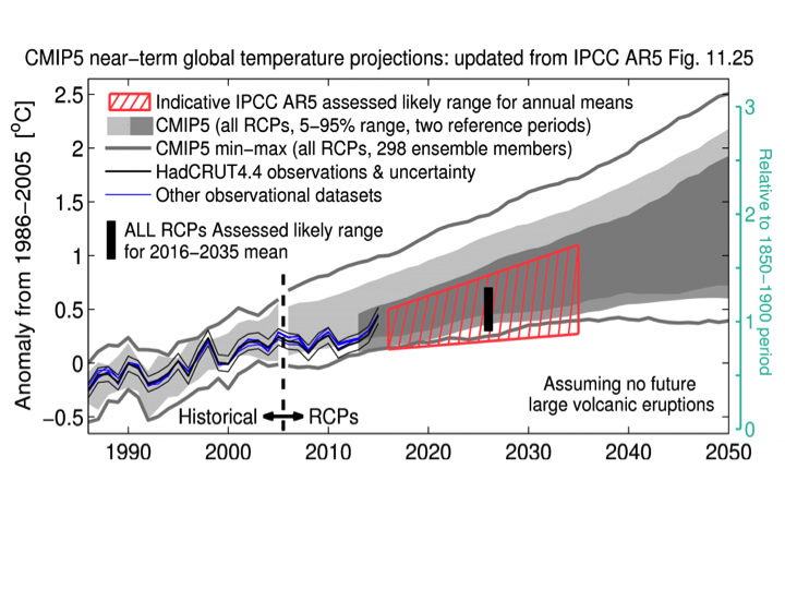
Chapter 11 of the IPCC AR5 Report focused on near term climate change, through 2035. Figure 7 compares climate model projections with recent observations of global surface temperature anomalies.Figure 4. Comparison of CMIP5 climate model simulations of global surface temperature anomalies with observations through 2014 (HadCRUT4). Figure 11.25 of the IPCC AR5
The observed global temperatures for the past decade are at the bottom bound of the 5-95% envelope of the CMIP5 climate model simulations. Overall, the trend in the climate model simulations is substantially larger than the observed trend over the past 15 years.
Regarding projections for the period 2015-2035, the 5-95% range for the trend of the CMIP5 climate model simulations is 0.11°C–0.41 °C per decade. The IPCC then cites ‘expert judgment’ as the rationale for lowering the projections (indicated by the red hatching in Figure 4):
“However, the implied rates of warming over the period from 1986–2005 to 2016–2035 are lower as a result of the hiatus: 0.10°C–0.23°C per decade, suggesting the AR4 assessment was near the upper end of current expectations for this specific time interval.”
This lowering of the projections relative to the results from the raw CMIP5 model simulations was done based on expert judgment that some models are too sensitive to anthropogenic (CO2 and aerosol) forcing.
IPCC author Ed Hawkins, who originally created the above figure, has updated the figure with surface temperature observations though 2015: Figure 5. Comparison of CMIP5 climate model simulations of global surface temperature anomalies with observations through 2014 (HadCRUT4). Updated from Figure 11.25 of the IPCC AR5, to include observations through 2014. http://www.climate-lab-book.ac.uk/comparing-cmip5-observations/
The spike in global temperatures from the 2015 El Nino helps improve the agreement between models and observations, but not very much. The 2015 temperature spike does not even reach the midpoint of the climate models, whereas the 1998 El Nino temperature spike was at the top of the envelope of temperature predictions. The bottom line conclusion is that so far in the 21st century, the global climate models are warming, on average, about a factor of 2 faster than the observed temperature increase.
The reason for the discrepancy between observations and model simulations in the early 21st century appears to be caused by a combination of inadequate simulations of natural internal variability and oversensitivity of the models to increasing CO2 (ECS). Multi-decadal ocean oscillations (natural internal variability) play a dominant role in determining climate on decadal timescales. The Atlantic Multidecadal Oscillation (AMO) is currently in its warm phase, with a shift to the cool phase expected to occur sometime in the 2020’s. Climate models, even when initialized with ocean data, have a difficult time simulating the amplitude and phasing of the ocean oscillations. In a paper that I coauthored, we found that most of CMIP5 climate models, when initialized with ocean data, show some skill out to 10 years in simulating the AMO. Tung and Zhou argue that not taking the AMO into account in predictions of future warming under various forcing scenarios may run the risk of over-estimating the warming for the next two to three decades, when the AMO is likely in its cool phase.
Projections for the year 2100
Climate model projections of global temperature change at the end of the 21st century are driving international negotiations on CO2 emissions reductions, under the auspices of the UN Framework Convention on Climate Change (UNFCCC). Figure 6 shows climate model projections of 21st century warming. RCP8.5 reflects an extreme scenario of increasing emissions of greenhouse gases, whereas RCP2.6 is a scenario where emissions peak around 2015 and are rapidly reduced thereafter.Figure 6: Figure SPM.7 of the IPCC AR5 WG1. CMIP5 multi-model simulated time series from 1950 to 2100 for change in global annual mean surface temperature relative to 1986–2005. Time series of projections and a measure of uncertainty (shading) are shown for scenarios RCP2.6 (blue) and RCP8.5 (red). Black (grey shading) is the modelled historical evolution using historical reconstructed forcings. The mean and associated uncertainties averaged over 2081−2100 are given for all RCP scenarios as colored vertical bars.
Under the RCP8.5 scenario, the CMIP5 climate models project continued warming through the 21st century that is expected to surpass the ‘dangerous’ threshold of 2°C warming as early as 2040. It is important to note that the CMIP5 simulations only consider scenarios of future greenhouse gas emissions – they do not include consideration of scenarios of future volcanic eruptions, solar variability or long-term oscillations in the ocean. Russian scientists argue that we can expect a Grand Solar Minima (contributing to cooling) to peak mid 21st century.
While the near-term temperature projections were lowered relative to the CMIP5 simulations (Figure 7), the IPCC AR5 SPM[2] states with regards to extended-range warming:
“The likely ranges for 2046−2065 do not take into account the possible influence of factors that lead to the assessed range for near-term (2016−2035) global mean surface temperature change that is lower than the 5−95% model range, because the influence of these factors on longer term projections has not been quantified due to insufficient scientific understanding.”
There is a troubling internal inconsistency in the IPCC AR5 WG1 Report: the AR5 assesses substantial uncertainty in climate sensitivity and substantially lowered their projections for 2016-2035 relative to the climate model projections, versus the projections out to 2100 that use climate models that are clearly running too hot. Even more troubling is that the IPCC WG3 report – Mitigation of Climate Change – conducted its entire analysis assuming a ‘best estimate’ of equilibrium climate sensitivity to be 3.0 oC.
The IPCC AR5 declined to select a ‘best estimate’ for equilibrium climate sensitivity, owing to discrepancies between climate model estimates and observational estimates (that are about half the magnitude of the climate model estimates). Hence the CMIP5 models produce warming that is nominally twice as large as the lower values of climate sensitivity would produce. No account is made in these projections of 21st century climate change for the substantial uncertainty in climate sensitivity that is acknowledged by the IPCC.
The IPCC’s projections of 21st century climate change explicitly assume that CO2 is the control knob on global climate. Climate model projections of the 21st century climate are not convincing because of:
- Failure to predict the warming slowdown in the early 21st century
- Inability to simulate the patterns and timing of multidecadal ocean oscillations
- Lack of account for future solar variations and solar indirect effects on climate
- Neglect of the possibility of volcanic eruptions that are more active than the relatively quiet 20th century
- Apparent oversensitivity to increases in greenhouse gases
There is growing evidence that climate models are warming too much and that climate sensitivity to CO2 is on the lower end of the range provided by the IPCC. Nevertheless, these lower values of climate sensitivity are not accounted for in IPCC climate model projections of temperature at the end of the 21st century or in estimates of the impact on temperatures of reducing CO2 emissions.
The IPCC climate model projections focus on the response of the climate to different scenarios of emissions. The 21st century climate model projections do not include:
- a range of scenarios for volcanic eruptions (the models assume that the volcanic activity will be comparable to the 20th century, which had much lower volcanic activity than the 19th century
- a possible scenario of solar cooling, analogous to the solar minimum being predicted by Russian scientists
- the possibility that climate sensitivity is a factor of two lower than that simulated by most climate models
- realistic simulations of the phasing and amplitude of decadal to century scale natural internal variability.
The climate modeling community has been focused on the response of the climate to increased human caused emissions, and the policy community accepts (either explicitly or implicitly) the results of the 21st century GCM simulations as actual predictions. Hence we don’t have a good understanding of the relative climate impacts of the above or their potential impacts on the evolution of the 21st century climate.
Filed under: climate models