by Frank Bosse
Separating out the impacts of internal variability on evaluations of TCR.
In a blogpost from May 2016 I did some simple investigations about the Transient Climate Response (TCR) as it’s observed. The starting point was the record of Cowtan/Way (C/W) and the Forcings due to greenhouse gases (GHG), land use and so on as they were described in IPCC AR5 . The result was a TCR for this record very near the TCR as it was determined by Nicholas Lewis from the HadCRUT4 record.
A few days ago Tamino (aka Grant Foster) released a blogpost with all the data (thank you for this, Tamino) in which he introduced a “sophisticated adjustment” to eliminate the influences of ENSO, solar TSI- changes and volcanic activities on the temperatures from 1951 to the present ( 8/2016) in many records. While there are several criticisms that can be made about this procedure, e.g. ENSO could be a part of the signal and not noise to eliminate, nevertheless I followed the method of Tamino. I was interested in using the records for the global mean surface temperatures (GMST) to recalculate the TCR as it was observed from 1951 to 2015 with annual data.
First, I made a figure of the adjusted temperature time series:
Fig.1: The adjusted time series of the Records GISS, HadCRUT4 (CRU), C/W and Berkeley. The difference between GISS and the average of the other three is shown in black.
GISS shows a higher warming in the adjusted record. The source of this discrepancy seems to be an additional positive trend from 1970 to 1988. After this year there is more or less a constant offset. The other three series are very close to each other. Only after 2005, the CRU series shows less warming (sea ice land/water?).
In a second step I do a linear regression of the forcings versus the adjusted surface temperature data from Tamino. This method does not equate to the formal definition of the TCR, although it has been used also in reviewed papers (see http://onlinelibrary.wiley.com/doi/10.1029/2008JD010405/full ); therefore it should be a good tool for a close approach. I excluded solar and volcanic forcings because their influences on the temperatures were also excluded by Tamino. For the case of C/W (as also shown in the former blogpost) the plot looks like this:
Fig.2: Linear regression of the AR5-forcing data versus the temperature anomaly in the series of C/W. The trend slope shows the warming due to a forcing: 1 W/m² gives 0.36 K warming.
For comparison: the “unadjusted” record as it was used in the May -blogpost:
Fig. 3: The regression of the unadjusted C/W series from 1940–2015. The result is almost the same, only one hundredth of a degree difference.
The only prominent difference is the bigger R²: In the adjusted time series in Fig. 2, the forcings account for 86% of the variance of the GMST, whereas in the unadjusted series it’s only 78%. This shouldn’t make us wonder: The volcanic and solar effects and also ENSO have no influence on the adjusted series –the adjustments work fine.
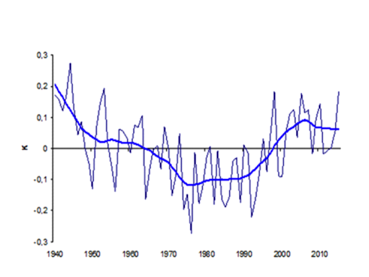
Now let’s also take a look at the residuals of the years to the linear trend line in Fig. 2:
Fig. 4: The residuals of the adjusted C/W series, which is the temperature variability not explained by the evolution of forcing with a 15 year smooth (Loess).
The same procedure from the May- blogpost gave this:
Fig. 5: The residuals for the unadjusted C/W series. The big (but short) ticks for volcanoes and ENSO ( see 1992/1993, 1997/1998) are not visible in fig. 4, however the long term pattern is not influenced by much.
The smoothed time series shows the same picture. Also after removing the volcanic and ENSO events, the internal variability remains almost the same. In the May blogpost I compared this pattern with the AMO (see Fig. 5 there) and the similarity seems to stand. The uptick between 1990 and 2005 is also clearly visible in the ENSO- adjusted series of Tamino. Therefore this low frequency internal variability has nothing to do with ENSO; it seems to be a result of the AMO.
In a third step I compared the records mentioned in Fig. 1. First, let’s have a look at the smoothed residuals:Fig. 6: The smoothed (15 years Loess) residuals of the linear regression of the GMST anomalies of the adjusted records versus the forcings.
The pattern is very stable in all records. The exception here is GISS. During 1970– 1995, the internal variability is dampened. A possible reason for this could be the ERSSTv4 adjustment during this period due to the change of the measurement methods (Karl et al. 2015); see also Fig. 1.
Finally I calculated the trend slopes of the 4 (adjusted by Tamino) records and the resulting TCR using the basic definition: a doubling of the CO2- content in the air generates a forcing of 3.71 W/m²The average TCR of the 4 records is 1.39 K/ 2*CO2. The average is heavily influenced by GISS, which shows some remarkable behavior in the residuals. The median of 1.35 K, which is less influenced by any one series, is probably a better measure. The R² of the linear trends of GMST versus forcings is for HadCRUT4; C/W; Berkeley; GISS: 0.86; 0.86; 0.88; 0.95. As higher the R² of the trend line as lower is the internal GMST variability of a given record.
Conclusions:
- The estimated TCR of ~ 1.35 (see Nicholas Lewis) is confirmed by the adjusted temperatures of the recent blogpost by Tamino. He stresses the physical importance of his statistical operation with the evaluation of his model.
- In contrast to the statement of Tamino that “there is a steady warming since 1976” with almost no variability, there is a decadal up and down in the adjusted time series very similar to the AMO-pattern with an amplitude of round about 0.2K .
- The TCR estimate from observations of ~1.35 is supported by at least 3 independent records: CRU, C/W and Berkeley with a deviation of only around 6%. The reason for the upward divergence of the GISS series associated with a suppressed internal variability can only be guessed. A closer investigation of this divergence is beyond the scope of this blogpost.
Moderation note: As with all guest posts, please keep your comments civil and relevant.
Filed under: Data and observations, Sensitivity & feedbacks