by Javier
Insights into the debate on whether the Holocene will be long or short.
Summary: Milankovitch Theory on the effects of Earth’s orbital variations on insolation remains the most popular explanation for the glacial cycle since the early 1970’s. According to its defenders, the main determinant of a glacial period termination is high 65° N summer insolation, and a 100 kyr cycle in eccentricity induces a non-linear response that determines the pacing of interglacials. Based on this theory some authors propose that the current interglacial is going to be a very long one due to a favorable evolution of 65° N summer insolation. Available evidence, however, supports that the pacing of interglacials is determined by obliquity, that the 100 kyr spacing of interglacials is not real, and that the orbital configuration and thermal evolution of the Holocene does not significantly depart from the average interglacial of the past 800,000 years, so there is no orbital support for a long Holocene.
Introduction
An understanding of past climate changes helps to put current global warming or “climate change” into perspective. Failure to account for past abrupt climate changes leaves us with a sample size of one warming and can cause a statistical type I error. When the village boy cried wolf, he was proposing an alternative hypothesis to the villagers. The null hypothesis was that there was no wolf. When the villagers accepted the boy’s hypothesis with a sample size of one and not enough evidence, they committed a type I error, a false positive. Given the risk of committing such an error with climate change, it is important to study the climate of the past.
Since there is only one reality and unlimited hypotheses to explain it, whenever confronted with a new claim, it is reasonable to think that the null hypothesis is it is not true. Adopting that reasonable position means being skeptical by default. That doesn’t make one very popular in the village, but makes one right most of the time.
Since extraordinary claims require extraordinary evidence, we raise the bar for evidence and lower the chance of rejecting the null hypothesis. In this way we reduce the chance of committing a type I error (reject the null hypothesis when it is true). The study of past climate changes is therefore of great importance in the study of the present global warming. A priori we should be skeptical about claims that “this time is different”, not because it is false, but because every time is different. Every interglacial period is different, but that does not mean that common explanations cannot be found, even if different factors were contributing in different ways to each of them. After all, science is a lot more about finding common elements to different observations than finding specific explanations to each observation.
In this series of articles, entitled “Nature Unbound: Climate Changes of the Recent Past” I am going to examine significant climate changes that have taken place since humankind evolved. In the first article we will review the glacial cycle. The second article will focus on the abrupt changes, known as Dansgaard-Oeschger events, that occurred in the last glacial period. We will place a special emphasis on the 50 -15 kyr BP (thousands of years before 1950) period. Future articles in the series will examine some evidence on the millennial cycles of the Holocene and some speculation about the future. I hope that in the process we can learn enough about climate change to add some perspective into the present one.
To set the stage we must know that the Earth has spent 90% of its time during the past million years in the coldest 1% of the temperatures seen in the past 500 million years. The Earth is locked in a very cold stage known as the Quaternary Ice Age. The reasons for this are unknown. An ice age is defined as any period when there are extensive ice sheets over vast land regions, as we see now. Since the last four ice ages have taken place roughly 150 million years apart, some scientists favor an astronomical explanation (changes in the Sun, the orbit of the Earth, or passage of the solar system through the galactic plane), while others prefer a terrestrial explanation (changes in the continental distribution, or concentration of greenhouse gases).
So, we don’t know why the Earth is in an ice age, but at least we think we know why 10% of the time the Earth gets a brief respite from predominantly glacial conditions and enters a milder condition known as an interglacial.
The glacial cycle. Milankovitch Theory.
The currently favored theory on glacial-interglacial climate change was first proposed in 1864 by James Croll, a self-educated janitor at the Andersonian College in Scotland, which goes to show that anybody can do science. He was offered a position in 1867, corresponded with Charles Lyell and Charles Darwin, and was awarded an honorary degree. But scientific knowledge at the time and his own limitations in mathematics and astronomy led to the final rejection of the theory. Croll wrongly concluded that orbital eccentricity and lack of winter insolation were responsible for glacial periods, and although he was the first to propose a positive ice-albedo feedback as a mechanism, his model called for asynchronous glaciations at the poles and timings for glaciations that were not supported by the then available (but incorrect) evidence.
The Serbian genius Milutin Milankovitch was, in 1920, the first to undertake the work of calculating the intricacies of the Earth insolation at different latitudes due to orbital variations in a time without computers, and he immediately identified summer insolation as a key factor to explain the drastic climate changes of the past. His theory was not accepted until 1970, when geological evidence was found on multiple glacial-interglacial cycles, although their timing (100 kyr) was a bit off relative to Milankovitch Theory. Proper dating of glaciations during the past 2.6 million years showed that for the most part they have taken place at intervals of 41,000 years, a period more akin to orbital insolation forcing.
Milankovitch Theory is very well known, so there is no point in going over it with much detail. Suffice to say that there are three types of orbital changes that affect Earth’s insolation over the long term (figure
Eccentricity: If the Solar system was only composed of the Sun and the Earth, Earth’s elliptical orbit would always have the same eccentricity, but as the movements of the other planets, specially the closest giants Jupiter and Saturn, introduce gravitational perturbations, the Earth’s orbit slightly changes its eccentricity. The eccentricity changes with a major beat of 413,000 years and two minor beats of 95,000 and 125,000 years. The changes in eccentricity are the only orbital changes that alter the amount of solar energy that the Earth receives as they change its distance from the Sun. Since the Earth’s orbit is always quite circular (eccentricity varies from 0.005 to 0.06) the change in insolation between Perihelion and Aphelion (now at January and July) is small, currently about 6.4% (0.016 eccentricity). The changes in eccentricity also produce a shortening and lengthening of the seasons as the Earth speeds at Perihelion and slows at Aphelion. Currently the northern Hemisphere winter (at perihelion) is 4.6 days shorter than southern Hemisphere winter (at aphelion). The important thing to remember in terms of climatic change is that due to the length of its main cycle, and the low eccentricity of Earth’s orbit, the eccentricity cycle results in an exceedingly small forcing. Or in other words, the insolation changes due to eccentricity are very small by themselves. It is only through its effect on precession and obliquity that eccentricity becomes relevant.
Obliquity: This cycle is given by the changes in the inclination of Earth’s axis, or axial tilt, with respect to Earth’s orbital plane. The axial tilt varies between 22.1° and 24.3° over the course of a cycle that takes 41,000 years. Currently the tilt is 23.44° and decreasing. The change in tilt changes the distribution of the solar energy between the seasons and through latitudes. The higher the obliquity, the more insolation in the poles during the summer and the less insolation in the poles during the winter and in the tropical areas all year. High obliquity promotes interglacials while lower obliquity is associated with glacial periods. While obliquity does not change the amount of insolation the Earth receives, it does change the amount of insolation each latitude receives and the change is large at high latitudes.
Precession: There are two precessional movements. The axial precession is the Earth’s slow wobble as it spins on its axis due to the gravitational pull on its equator by other solar bodies. The Earth’s axis then describes a circle against the fixed stars in 26,000 years, so if it is now pointing to Polaris, 13,000 years ago it was pointing to Vega. The orbital (or apsidal or elliptical) precession is the slow rotation of the elliptical orbit around the focus of the ellipse closest to the Sun in a period of 113,000 years. The combined precession (of the equinoxes) displaces progressively the seasons around the year and around the orbit, so that if now northern Hemisphere winter takes place at perihelion (perigee closest to the Sun), in about 11,500 years it will be taking place at aphelion (apogee farthest from the Sun). Precession is therefore modulated by eccentricity as the precession angle would be irrelevant at zero eccentricity (circular orbit). It is important to note that precession doesn’t change the amount of insolation that the Earth receives or the amount of insolation that each latitude receives during the year. Whatever insolation precession gives to one season, it takes it back from the other seasons, thus precession is an important contributor to summer insolation and to the insolation latitudinal gradient. The interaction of the various components of precession produce cycles at 19, 22 and 24 kyr with a mean period of roughly 23,000 years. Since the northern hemisphere summer now takes place at aphelion, we are at a minimum, in the precessional cycle, from the point of view of summer insolation at 65°N.
Figure 1. Changes in Earth’s orbit as the basis for Milankovitch theory. The orbital eccentricity variation (green) produces changes in the shape of the Earth’s orbit with periods of 413 kyr and 100 kyr. Axial tilt (blue) changes with obliquity periods of 41 kyr. The orbital precession (orange) rotates the orbit around one of the elliptical foci, while the axial precession (yellow) wobbles the Earth. Both together produce an average period of 23 kyr. Source: Cyril Langlois
As currently viewed by followers of Milankovitch Theory, glacial inception takes place when the summer insolation at 65°N allows more ice to survive the summer every year. This starts the buildup of the Laurentide, Fennoscandian and Siberian ice sheets. This process is fueled by ice-albedo and other feedbacks and progressively cools the Earth with a simultaneous drop in sea level. The glacial period survives several cycles of increased 65°N summer insolation and progressively gets colder and sea level lowers. The next eccentricity cycle, between 95 and 125 kyr later, induces a non-linear response on precession such that the next rise in 65°N summer insolation triggers a glacial termination. This is a much faster process than glaciation as is helped by feedback effects such as a reduction in ice-albedo or a buildup of greenhouse gases.
Glacial cycles are a tough nut to model with current climate models which are built using Holocene conditions. The discussions between Milankovitch defenders are about the fashionable role of CO2 in glacial termination (Shakun et al., 2012), about a three stage model with interglacial, mild glacial and full glacial conditions (Paillard, 1998), or about a sea-ice switch to explain why other peaks in 65°N summer insolation fail to get the world out of a glacial until the eccentricity cycle kicks in 100 kyr later (Gildor and Tziperman, 2000).
Problems with Milankovitch Theory
The current theory explaining glaciations through summer insolation at 65°N, paced by the 100 kyr eccentricity cycle is supported by the scientific consensus and is presented in textbooks. But, it has some important holes that challenge its validity.
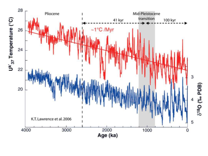
The most important one is the 100 kyr problem. Until about 1 million years ago glaciations were taking place at 41 kyr intervals, pointing to obliquity as the main factor. But since about that time glaciations have taken place at 100 kyr intervals (figure 2). When this was discovered the problem was that the Milankovitch Theory did not reserve any special place for the eccentricity cycle, since its effect is minimal. So Hays, Imbrie, and Shackleton in their 1976 article proposed that the eccentricity was playing its role in a non-linear way. The problem is compounded because the main cycle of eccentricity is 413 kyr and that cycle is even less apparent in the record so we are left with the conclusion that eccentricity produces a multiplicative effect during its minor cycles, yet no important effect in its major cycle. Maslin and Ridgwell (2005) call it “the eccentricity myth.” In addition, the change from early-Pleistocene 41 kyr glaciations to late-Pleistocene 100 kyr glaciations was achieved without any change in insolation, so Milankovitch Theory is at odds to explain it.
Figure 2. The Mid-Pleistocene Transition. Two different proxies for temperature, the alkenone UK’37 in marine sediments (red), and δ18O isotope in benthic cores (blue), show the progressive cooling of the Earth through the Pliocene. At the early- Pleistocene glaciations start to take place at 41 kyr intervals. As the cooling progresses, this interval lengthens to 100 kyr in what is called the Mid-Pleistocene Transition or Revolution. Source: K.T. Lawrence, et al. 2006.
The 100 kyr problem is best illustrated in figure 3 where we compare the Milankovitch Theory, through the decomposition of the insolation into its components: eccentricity, obliquity and precession (figure 3 A); with evidence from temperature proxy records (figure 3 B), through frequency analysis to reveal their main cyclic components. Note that you rarely see eccentricity plotted at its true comparative forcing. The disparity is so evident that the current consensus glacial cycle hypothesis cannot be right.
Figure 3. The 100 kyr problem. Milankovitch theory, in its current consensus form, runs into problems explaining the disparity between predictions and observations. A. The calculation of 65°N summer insolation shows that the predicted range of 105 W/m2 is mainly due to the contribution of precession, followed by obliquity with a similar magnitude. The contribution from eccentricity is however very small. B. When the spectra of the temperature proxies is analyzed, the main band is a 100 kyr band, followed in intensity by a 41 kyr band, while the 23 and 19 kyr bands are barely detectable. So, the strongest contributor gives the weakest signal, while the strongest signal comes at a frequency of what should be a negligible contributor. Source: J. Imbrie et al. 1993. Modified.
Second in importance is the causality problem, exemplified in “the stage 5 problem.” Marine Isotope Stage 5 is used here as an alternative name for the previous interglacial, also known as Eemian in North America. According to insolation, the Eemian or MIS 5 should have started at the earliest 135 kyr BP, however data from crystals in a Nevada cave named Devils Hole in 1992 indicate that by that date glacial termination was essentially finished (Winograd et al., 1992; Ludwig et al., 1992; Glacial termination is defined as the midpoint in sea level between glacial and interglacial). A great controversy erupted over that data in the literature and has not abated since. But Devils Hole data is not alone, as similar data has been uncovered from coral reefs in the Bahamas (Gallup et al. 2002), Barbados and Papua New Guinea, and from Iberian-margin sediments and Italian cave speleothems (Drysdale et al. 2009), and all of it indicates that termination was essentially completed by 135 kyr BP. A date when 65°N summer insolation was still below the levels of 70% of the previous 100 kyr (figure 4). Additional data indicates that MIS 5 may not be the only glacial termination where the effect appears to precede the cause. MIS 15c shows the same situation. The problem is further complicated because summer insolation has been used as a defining criterion to date the start and end of glaciations in sediments in the official UN sponsored SPECMAP series. This results in circular reasoning since computed insolation is assumed to pace the glaciations and terminations and has been used to date them.Figure 4. The causality problem. The arrow marks when the effect has taken place before the theoretic cause. According to Milankovitch theory, glacial termination II, leading to MI Stage 5 or the Eemian interglacial, could not have commenced earlier than 135 kyr ago (vertical grey dotted line) due to lack of solar forcing. However, data from Devils hole cave (thin grey line) indicates a much earlier start since deglaciation was already well under way at 140 kyr ago. SPECMAC series data (thick black line) is of no help since it was set to match 65°N summer insolation so the middle of each rise is set at maximum insolation (grey vertical bars). Data from Barbados coral reefs (Green and yellow) supports the early start as sample NU-1471 indicates that by 136 kyr ago, according to sea levels, termination II was already 80% complete. The 65°N summer insolation is in orange. Obliquity is in blue. Obliquity cycle started 10 kyr earlier, at 150 kyr ago. Source: C.D. Gallup et al. 2002. Obliquity added.
A third issue is that glacial cycles are symmetric between the hemispheres, as both are warming or cooling simultaneously, whereas the seasonal precession forcing (and 65°N summer insolation) is anti-symmetric. That is when one hemisphere warms, the other cools.
A fourth problem that is seldom discussed is the 41 kyr problem (Raymo and Nisancioglu, 2003). If Milankovitch Theory struggles to explain the glacial cycle in the last 0.8 million years, it has no less problems to explain it between 3-0.8 million years ago. During that period temperatures and global ice volume varied almost exclusively at the 41 kyr obliquity period, while high-latitude summer insolation is always dominated by precession. Raymo and Nisancioglu (2003) argue that these earlier interglacials cannot be understood within the current framework of the Mylankovitch Hypothesis.
Evidence that the pacing of interglacials does not follow a 100 kyr cycle
The claim that interglacials follow a 100 kyr cycle is surprising. According to the LR04 marine sediment core or EPICA Dome C Antarctic ice core no single interglacial of the past 800,000 years starts 100,000 years after the previous one (table 1). It is also difficult to understand how a 100 kyr cycle hypothesis can be supported based upon 11 interglacials within the last 800 kyr that have an average spacing of 72.7 kyr, very far from 100.
Table I. Interglacials of the past 800,000 years. Interglacial start date was determined directly from EPICA Dome C temperature data from δDeuterium isotopic changes. Temporal distance between interglacials was calculated between start times. Average distance is 72.7 kyr, while most frequent distance is close to 82 kyr.
To clarify this issue, I have plotted the interglacial start date versus distance from previous interglacial, following Euan Mearns (The Alpine Journal, in press; personal communication). The result is given in figure 5. The data strongly indicates that the spacing of interglacials tends to fall on multiples of the 41,000 year obliquity cycle. There are two anomalous interglacials, MIS 11 was unusually long, and MIS 7e was unusually short. If their deviation is due to an early start in the first case and a late start in
the second, then the distance to the next interglacial might be affected simply by the change in start date. Correcting for the start date, the length of the two interglacials places every cycle in the graph close to the obliquity lines.
Figure 5. The 100 kyr Myth. Plot of Interglacial start date versus distance to the previous interglacial. The spacing of interglacials shows a strong tendency to fall into multiples of obliquity spacing (red bands). Even the anomalous interglacials MIS 11 and MIS 7e (stars) can be explained by their abnormal length. If their length transgressions were accounted for, every dot would be near the red bands. Bottom: EPICA Dome C temperature plot. Grey continuous line, obliquity. Grey dotted line, eccentricity.
Another observation is the presence of two interglacials separated by only one obliquity cycle (41 kyr) at times of very high eccentricity (figure 5). This suggests the existence of a repeating pattern following the 413 kyr eccentricity cycle where the length of a unit is given by the distance between MIS 15a and MIS 7c, 365,000 years, or nine obliquity cycles, during which five interglacials take place, four of them separated by 82 kyr and one by 41 kyr. The average spacing of interglacials would then be 73 kyr, very close to the average value of 72.7 kyr for the entire series. Interglacials would take place every 1.8 obliquity cycles, although the cycle is irregular, as the existence of short and long interglacials and the past glacial period lasting three obliquity cycles show.
Evidence that obliquity and not insolation sets the pacing of interglacials
The evidence that obliquity sets the pace of interglacials is so abundant and clear; I am very surprised by the general failure to recognize it, even by scientists and people that have looked at the data in detail. Since Milankovitch proposed that the pace of interglacials was set by changes in insolation forcing caused by orbital variations, the belief in the climatic effect of summer insolation variations at 65°N is deeply ingrained. It is questioned by few, and reminds us of other hypotheses that are taken as fact without solid evidence. Let’s review the evidence in favor of obliquity:
a) Glacial cycles were indeed governed by the 41 kyr obliquity cycle for most of the Quaternary Ice Age prior to the mid-Pleistocene transition (figures 2 and 6), and the 23 kyr and 100 kyr cycles werenowhere to be seen in that period. The simplest “Occam’s razor” explanation is that obliquity does the job.
b) Throughout the Pleistocene, Earth has been cooling down progressively (figure 2). The cooling of the planet reached a point at around 5 million years ago when some interglacials started to be affected and did not reach what we consider interglacial temperatures, so we do not consider them to be interglacials and do not assign them numbers in the MIS sequence (figure 6, asterisks). However, the Mid-Pleistocene Transition did not involve any change in insolation, or orbital cycles, so proponents of the 100 kyr-Insolation Milankovitch Hypothesis are at odds to explain how an obliquity cycle turned into an eccentricity cycle.
Figure 6. Pleistocene temperature proxy record. δ18O isotopic record from LR04 stack of 53 benthic cores from all over the world shows that from about 1.5 million years ago some interglacials continued reaching the previous average temperature (red line), while others show a decreasing trend in interglacial average temperature (blue line), and are not considered interglacials. Periods of higher temperature more recent than MIS 23 that did not reach interglacial levels are usually not assigned an MIS number (asterisks). Source: Lisiecky and Raymo, 2005.
The most interesting question is not why some obliquity induced periods of warming fail to reach what we consider interglacial temperatures, but why some still manage to reach them given the cooling of the planet.
c) Although precessional changes greatly affect the amount of insolation during a three-month period, that change is quickly averaged over the following three months, leaving total annual radiation unchanged. By contrast obliquity changes add a significant amount of warming at high latitudes year after year over a period of thousands of years and can have an enormous cumulative effect (figure 7). The temperature proxy record clearly shows temperatures decreasing during periods of low obliquity (yellow at mid-latitudes in figure 7), and increasing during periods of high obliquity (blue at mid-latitudes in figure 7).
Figure 7. Annual insolation changes at high latitudes and the symmetry problem. Changes in annual insolation by latitude and time are shown in a colored scale. They are essentially due to changes in obliquity (blue sinusoidal curve), since changes in insolation by precession are averaged between seasons within the same year. The high latitude persistent changes in insolation last for thousands of years and correspond quite well to changes of temperature in Antarctica, shown as a blue line overlay. Glacial-interglacial cycles show symmetric temperature responses in both hemispheres. As we can see Antarctic temperatures respond with warming despite 65°N summer insolation increases corresponding to 65°S summer insolation decreases. Source: Steve Carson. The science of Doom.
d) Summer insolation is dominated by the 23 kyr precession cycle. When a frequency analysis is performed on both the insolation calculated data and on temperature proxy data only a very small response from temperatures to insolation is detected (figure 8). The only consistent response between both insolation and temperature data is given by Not only is there no significant signal for a 23 kyr cycle in the data, but if 65°N summer insolation is so important it becomes difficult to explain why it sometimes has a huge effect on temperatures and at other times it has almost no effect.
Figure 8. Disparity between calculations from Milankovitch theory and data from observations. A Gabor transform is a windowed time-frequency Fourier analysis. When applied to the 65°N summer insolation calculations from the orbit of the Earth during the last 800 kyr it shows the main contributors to that signal thought to be responsible for glacial terminations. The main contributor is the 23 kyr period, followed by the 18 kyr period, both from precession cycles, followed by the less intense 41 kyr period from obliquity cycles. When the same analysis is performed over the temperature data from observations (Epica Dome C ice core record), we can see that the temperature of the Earth barely responds to precession, as the band at 23 kyr is very tenuous. Instead we see obliquity bands at 41 and 83 kyr (double harmonic) and the prominent band at 100 kyr, that cannot be the eccentricity, since it is missing what should be an even stronger band at 413 kyr. Source: John Baez.
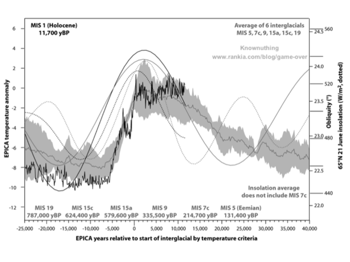
e) When six interglacials of the past 800 kyr that display a similar duration, plus the Holocene, are aligned by temperature, their obliquity graphs also align (figure 9). The change in obliquity and temperatures is in phase with a delay. However, the same is not true for their insolation pattern, that displays more variability (figure 10). This variability underscores that for MIS 7c, MIS 5, and MIS 15c insolation could not have driven glacial terminatio In the first interglacial insolation was too early and the last two it was too late (see the stage 5 problem above).
Figure 9. Interglacial alignment with obliquity. Interglacials MIS 1, 5, 7c, 9, 15a, 15c, and 19 were aligned by temperature. Their obliquities also display a significant degree of synchronization. Obliquity bottoms 20 to 15,000 years before the start of the interglacial. The warming in Antarctica starts about 10,000 years later, and proceeds so fast that interglacial average temperatures are reached by the time obliquity peaks about 19,000 years after it started rising. The interglacial comes to an end with a delay of about 5,000 years over the falling obliquity. Sources: EPICA Dome C, Jouzel, J., et al. 2007. Astronomical data, Laskar, J., et al. 2004.
Figure 10. Interglacial alignment with 65° N summer insolation. Same as figure 9 for northern summer insolation. Although insolation also has a tendency to align indicating that interglacials cannot take place if insolation is working in the opposite direction, the spread is clearly higher in this case. Insolation for MIS 7c came too early and for MIS 15c and MIS 5 too late to be held responsible for driving interglacial warming.
f) Average duration of MIS 5, 7c, 9, 15a, 15c, and 19 interglacials measured at the -3° C anomaly in the EPICA data is ~ 18,000 years. Average duration of the up swing of the obliquity cycle at 23.5° is ~18,000 years. Average duration of the northern summer insolation cycle at 500 W/m2 is ~ 11,000 years.
Interglacials tend to last the same as the obliquity cycle but shifted 4-6,000 years due to the Earth’s thermal inertia. It is the same reason that makes the yearly temperature cycle follow the seasonal insolation cycle with about a 1.5 month delay.
Evidence from interglacial pacing, temperature response to obliquity, temperature-obliquity alignment, and interglacial average duration clearly indicates that, in general, interglacials respond primarily to the obliquity cycle as they have always done and still do. Despite a general consensus ignoring what the data clearly indicates, some authors have realized this fact and are proposing hypotheses where obliquity is responsible for the glacial cycle (figure 11. Huybers and Wunch, 2005; Huybers, 2007; Liu et al., 2008).
Figure 11. A simple stochastic model of glacial-interglacial cycles based on obliquity. Huybers and Wunch, 2005, could not statistically reject the null hypothesis that glacial terminations are not caused by precession or eccentricity, but rejected that they were not caused by obliquity. They developed a model based only on obliquity that reproduced the pacing observed. Left, A run of the model. Right, frequency histogram of the glacial duration of multiple runs of the model showing the duration of the past 6 glacial periods as black triangles. Source: Huybers and Wunch, 2005.
The hypothesis that obliquity drives the glacial cycle solves most of the problems of Milankovitch Theory. The 100 kyr problem is solved because there is no 100 kyr cycle, just a 41 kyr cycle that skips one or two beats. And it solves the 41 kyr problem for similar reasons. It solves the causality problem because now glacial terminations usually start at the bottom of the obliquity cycle and therefore MIS 5 termination is well underway at 135 kyr BP when 65°N summer insolation is still too low. It also solves the lack of asymmetry in the polar response, as the obliquity cycle is symmetrical in both poles.
Interglacial determination in the Late Pleistocene
Knowing that obliquity is the main factor in enabling and pacing interglacials also in the Late Pleistocene, we can analyze the data to see which other factors contribute to determine when an interglacial should start. Interglacials take place after a period of increasing obliquity, and there have been 24 such windows of opportunity during the past million years, producing 13 interglacials and 11 obliquity cycles without an interglacial. Figure 12 shows those windows of opportunity (numbers on top) with red bars for the successful ones and blue bars for the unsuccessful. Two factors can be identified as being important. The first one is 65°N summer insolation above 520 W/m2 at the second half of the opportunity window (above the red line, red and green circles in the insolation panel of figure 12), and the second one is temperatures at or below those equivalent to 4.55 ‰ δ18O or above at the first half of the opportunity window (below the blue line, red circles in the temperature panel of figure 12).
When temperatures are high at the start of the window of opportunity and insolation does not reach 520 W/m2 towards the end, the interglacial does not take place despite increasing obliquity. When one of the conditions is right but the other is not, the best prediction is given by the low temperature condition, as most of the time a low enough temperature at the start of the rising obliquity drives an interglacial even if insolation is not high towards the end of the rising obliquity. High insolation at the end of the obliquity window alone does not result in an interglacial unless it is extremely high, above 550 W/m2, and this only happens when eccentricity is very high, 200, 600 and 1000 kyr ago (green circles and green numbers in figure 12). This is the likely reason why interglacials have a reduced spacing of one obliquity cycle (41 kyr) at times of peak eccentricity, as in the case of MIS 15a/MIS 15c and MIS 7c/MIS 7e.
Figure 12. A simple model of interglacial determination based on obliquity, insolation, and temperatures. Top, A window of opportunity takes place every time obliquity increases, marked with a colored bar, red when an interglacial results and blue when not. Middle, Insolation is proposed to promote interglacial conditions when above the red dashed line at 520 Wm2, during the second half of the window (red circles), or directly result in an interglacial when above the green dashed line at 550 W/m2(green circles). Bottom, Low temperatures are proposed to promote interglacial conditions when below the blue dashed line at 4.55 ‰ δ18O during the first half of the obliquity window (red circles). Numbers on top are periods of increasing obliquity with red numbers indicating an interglacial produced by favorable conditions (red circles), blue numbers indicate an interglacial was not produced due to unfavorable conditions (blue circles), and green numbers indicate interglacials produced by very high insolation despite unfavorable temperatures (green circles). MIS 13 (window 13) cannot be explained by this model, thus the question mark.
MIS 13 cannot be explained in terms of insolation and initial temperature conditions like the rest of interglacials. It is a very atypical interglacial. Temperatures were very high at the start of the obliquity increase, so instead of a rapid warming driven by strong feedbacks, its warming is progressive and relatively slow. It does not align with the rest due to its unusual temperature profile, complicating our analysis. It looks like a failed interglacial with a big temperature spike towards the end.
The low temperature factor at the start of the obliquity increase is clearly a proxy for strong feedback factors that operate more strongly when temperatures are very low. Among the known factors are:
- – Reduction of ice-albedo
- – Increased melting of ice
- – Rising sea levels
- – Increase in dust
- – Increase in greenhouse gases
The effect of the temperature decrease during a glacial period prior to the next obliquity cycle has the effect of pulling a spring. The stronger it is pulled, the stronger and faster it will go in the opposite direction when released. This spring acts as a negative feedback to further cooling, and its existence could be inferred from the narrow thermal regulation of the planet during at least the past 560 million years. It is what allows interglacials to take place during this very cold period of the planet, as otherwise for the last 1.5 million years the planet would have been locked in a permanent glacial period only interrupted by interglacials every 400 kyr, at the peak of eccentricity. It is possible that there wouldn’t be humans in that planet as conditions are already too close to CO2 starvation for plants during glacial maxima. Only the arrival of the occasional interglacial prevents further cooling.
When obliquity starts rising during a glacial period it starts moving energy little by little from tropical to polar areas. Its effects on global average temperatures are not noticeable for many thousands of years. If the planet is very cold, with a great portion of the water in huge ice sheets over continents and continental shelves then powerful feedbacks will start. Temperatures will rise after about ten thousand years of increasing energy transfer to higher latitudes and warming will accelerate. It is at about this time when rising precessional insolation during the summer in the northern hemisphere will start contributing to the undergoing melting of the northern ice sheets. The contribution of feedback factors and northern summer insolation is what allows the Earth, every 1.8 obliquity cycles, to overcome the cold inertia of the planet. It is an additive process where obliquity sets the pace, and is helped by feedback factors and northern summer insolation. If one of these two is strong enough the other might be dispensed. The result is that every interglacial is different. It is the response to forces that assemble and come apart at different times and with different intensities.
An interglacial therefore can be predicted by knowing the temperature at the beginning of the obliquity cycle increase and the insolation conditions during the second half of the obliquity increase. As temperatures usually require more than one obliquity cycle to get low enough, that is the likely reason that interglacial spacing is close to two obliquity cycles. It is very unlikely therefore that a new interglacial will take place in 30,000 years, and more probable that it will take place in 70,000 years. In fact, an interglacial should have started 50,000 years ago, and we should not be in an interglacial now, but despite low enough temperatures (figure 12 number 2), insolation was very low at the time and started decreasing when obliquity was still rising.
Interglacials of atypical duration and the likely length of the Holocene
Six interglacials out of the past ten during the last 800 kyr display a very similar temperature profile in EPICA Antarctic records (MIS 5, 7c, 9, 15a, 15c, 19). They show a fast increase in temperatures for 5-7,000 years, followed by a temperature stabilization for about 5,000 more years, and then a slow temperature decline that accelerates with time for the next 10-12,000 years during which they lose two thirds or more of the temperature gained from the glacial maximum at the interglacial start. During the period of high temperatures (above -2° C anomaly), that lasts about 15,000 years, each interglacial presents a different temperature profile, highlighting interglacial uniqueness.
After aligning them, I have averaged the temperatures and obliquity of those six interglacials, and the insolation profile of five of them. MIS 7c presents a very deviant insolation profile that would significantly alter the average of the rest, so it was not included. The result is an average interglacial that we can compare to the two interglacials that display a very different duration, the short interglacial MIS 7e 244 kyr ago, and the long interglacial MIS 11 425 kyr ago (figure 13).
Figure 13. Comparison of atypical interglacials to the average interglacial. An average interglacial (grey curve and 1σ grey bands) was constructed from interglacials MIS 5, 7c, 9, 15a, 15c and 19, after aligning them at the specified date for each of them. The obliquity for all of them (grey sinusoid continuous line) and the insolation curves at 65° N 21st June for all but MIS 7c (grey dotted line) were also averaged. MIS 7e temperature, obliquity and insolation data are similarly plotted in blue, and MIS 11 in red. Sources: EPICA Dome C, Jouzel, J., et al. 2007. Astronomical data, Laskar, J., et al. 2004.
MIS 7e started very late in the obliquity cycle because most of the time when obliquity was increasing, northern summer insolation was decreasing (figure 13). Under normal circumstances MIS 7e would have been a cycle without interglacial, however 250 kyr ago eccentricity was very high and rising quickly (figure 5), and when at the obliquity maximum, insolation started to increase strongly, temperatures responded triggering a delayed interglacial. But as soon as insolation peaked 242 kyr ago, the simultaneous falling of obliquity and insolation could not sustain the interglacial. MIS 7e started late because it was triggered by the insolation cycle due to high precession, but ended on schedule for the obliquity cycle and became a shortened interglacial.
MIS 11 was also started by precessional insolation before obliquity had a chance to increase, becoming an early interglacial (figure 13). But the reason is not the same as MIS 7e, as precession was actually very low 430 kyr ago. If the relatively small increase in insolation provided the signal for glacial termination, the strength of MIS 11 early warming appears to have been provided by very strong feedback factors, as temperatures before MIS 11 appear to have been extremely low, the second lowest in the entire 5 million year LR04 benthic stack proxy (figure 12). MIS 11 became such long interglacial because it increased temperatures in three steps. The first step triggered by rising insolation and strong feedback response ended early when insolation peaked 244 kyr ago. But then rising obliquity provided the impetus for a second warming period, as insolation did not decrease much, that ended 235 kyr ago when obliquity peaked. Then a third warming step took place caused by a second insolation peak 226 kyr ago. The three warming steps responsible for the extraordinary duration of MIS 11 are clearly detected in the temperature record (see figures 5 and 13) and give MIS 11 the opposite temperature profile to most interglacials since it evolves from lower to higher temperatures. It is the interglacial with highest temperatures for the longest time despite occurring at a time of low eccentricity. Given the high increase in energy and the normal thermal inertia of the planet, its decline was also a very long one, despite being more pronounced than the average decline (figure 13).
Since both MIS 7e and MIS 11 were atypical interglacials and the product of very special circumstances, it is clear that scientists claiming that MIS 11 is a good analogy for the Holocene have not carefully examined the data, and are trying to make a rule out of an exception. Alignment of MIS 1 with the average interglacial shows that the Holocene is just another average interglacial (figure 14). The Holocene temperature profile is within one standard deviation of the average. Its obliquity profile exactly matches the average obliquity profile, and its insolation profile is slightly ahead of the average, but well within the variability for this parameter. The characteristics of the Holocene are a colder starting point because the glacial period that preceded it was the longest on record and the presence of the Younger Dryas, a hiccup in the fast warming phase of unknown origin. Although I recently proposed that a low in the ~ 2400 yr Bray solar cycle at a sensitive time might have contributed to it (Javier, 2016). Its colder start, slightly earlier increase in northern summer insolation, and the Younger Dryas explain why the Holocene has not been as warm as the Eemian.
Figure 14. Holocene comparison to the average interglacial. The average interglacial described in figure 13 (grey curve and 1σ grey bands) and the average obliquity (grey sinusoid continuous line) and insolation at 65°N on 21 June (grey dotted line) are compared to Holocene temperature (smoothed, black curve), obliquity (black sinusoid continuous line), and insolation (black dotted line).
The conclusions drawn by comparing the Holocene to the average interglacial are the same as those obtained by comparing it to its closest astronomical analog, MIS 19 (Pol et al., 2010; Tzedakis et al., 2012). MIS 19 was an interglacial that was at the same “Milankovitch point” as our Holocene interglacial 777 kyr ago. It has an almost identical astronomical signature (figure 15), with the same low eccentricity and the same coincident peaks of precession and obliquity. The comparison suggests that the descent into the next glacial should start in about 1,500 years (Tzedakis et al., 2012). Notice also the natural warming events, known as AIM (Antarctic Isotope Maxima), that took place on a millennial scale.
Figure 15. Detailed comparison of the Holocene and MIS 19. a) δD (‰) temperature proxy of Holocene (red); b) MIS 19 δD (‰) mean signal (black). In panels a) and b) the thin dashed horizontal lines correspond to the present-day (last millennium average) δD levels; e) Eccentricity (dashed, right axis) and North Hemispheric 21 June insolation (solid, left axis); f) Climatic precession parameter (dashed, right axis), inverted, and finally obliquity (°, solid, left axis). AIM, Antarctic Isotope Maxima, a warm event. ACR Antarctic Cold Reversal. Source: Pol, K. et al., 2010.
Once the present short warming interval ends, the Holocene should continue its temperature descent and an increase in northern summer insolation in the next several thousands of years should not significantly alter this decline as it has not done so in the past (figure 10). To my knowledge no decaying interglacial has been revived this late in the obliquity cycle regardless of the amount of northern summer insolation. Therefore, there is no astronomical reason to expect that the Holocene should be a long interglacial, and humankind must wait for another obliquity cycle, probably the one after next, in 70,000 years, to have another chance at being scared by global warming.
Role of obliquity in the glacial cycle
Most scientific authors publishing on the glacial cycle have focused on local conditions to try to explain it. Insolation, albedo changes, and dust deposition are supposed to act maximally at a certain latitude at the edge of the ice sheet. Solving the glacial cycle however may require out of the box thinking. Raymo and Nisancioglu (2003) have proposed a “gradient hypothesis” to explain the role of obliquity during the Early Pleistocene. Orbital data indicates that the insolation gradient also changes in anti-phase with obliquity (figure 16). The insolation gradient is largely responsible for the equato-polar thermal gradient, that is widely believed to be the engine that drives heat and humidity transport from the equator to the poles through oceanic currents and the atmospheric circulation.Figure 16. Obliquity comparison to the insolation gradient. Insolation gradient curve (red) is the difference in summer half- year insolation between 25° and 70°N insolation. Minima in insolation gradient correspond to maximum obliquity (black). Source: M. E. Raymo & K. Nisancioglu, 2003.
The gradient hypothesis proposes that as obliquity and polar insolation increase, the insolation gradient decreases (figure 16). This would have the double effect of keeping more heat in the planet from being lost at the poles through radiation, and reducing the moisture poleward transport that feeds the ice sheets. The opposite effect would take place when obliquity decreases at the end of an interglacial. Within this hypothesis the tropics, with their huge thermal and moisture capacity, become principal agents in the formation and waning of ice sheets orchestrated by obliquity changes, while local factors like latitudinal insolation, albedo, and dust are important secondary players that sometimes become decisive.
Raymo and Nisancioglu (2003) have failed to extend their hypothesis to the Late Pleistocene, but there is no reason why the mechanisms involved should have changed at the Mid-Pleistocene Transition.
Role of CO2 in the glacial cycle
As evidence shows, authors that predict an unusually long interglacial continuing for 20 to 50 kyr longer (Loutre and Berger, 2000), based on 65°N summer insolation are mistaken. Astronomical data does not support a long interglacial. MIS 11 is the only example of a long interglacial in the Late Pleistocene (last 800 kyr), and has a unique astronomical configuration as shown above (figure 13).
Other authors however propose a long interglacial of 500 kyr (Archer and Ganopolski, 2005), tempered in a later article to just 100 kyr (Ganopolski et al., 2016), based on CO2 levels. The difference of half an order of magnitude in their calculations attests to the level of uncertainty in their estimates. Tomorrow may well be a date for the next glacial inception, as it is within their uncertainty bounds. But, the first thing they must do is to demonstrate that CO2 plays a significant role in the glacial cycle.
CO2 is no doubt one of the several feedbacks that must act on the glacial cycle, as CO2 levels increase with the warming of glacial terminations and decrease with the cooling of glacial inceptions. However, we must remember that CO2 is a positive feedback as it acts in the direction of the change in temperatures. The glacial cycle is clearly dominated by negative feedbacks that constrain temperature variations and as we have seen warming is faster with a colder starting temperature. This effect is clearly illustrated in figure 12 where the biggest warming responses belong to the coldest starting points, instead of being proportional to the amount of insolation increase.
Regarding CO2, we are confronted by an interesting paradox. We know from ice core measurements that glacial termination I (the closest to us 15 kyr ago) involved a change in CO2 atmospheric concentrations from 190 ppm to 265 ppm, an increase of 75 ppm. Concurrently the temperature increased globally by an estimated 4-5°C (von Deimling et al., 2006; Annan and Hargreaves 2013). The defenders of CO2 as a main factor in climate change have developed the hypothesis that CO2 was largely responsible for the warming at the end of glacial periods once the astronomical signal initiated the warming. But if CO2 carried out most of the warming, that means that at the very least more than 2°C of the warming was caused by the increase in CO2.
A simple calculation tells us that the rise from 190 to 265 ppm is 48% of a doubling of the temperature effect. This is true because we are dealing with a logarithmic scale, (ln(265)- ln(190))/(ln(190×2)-ln(190))=0.48). So 48% of a doubling produced at least 2°C of warming between 15-10 kyr ago. The rise from preindustrial to current levels of CO2 (280 to 400 ppm, or 120 ppm) constitutes 51% of a doubling of the temperature effect. That is (ln(400)-ln(280))/(ln(280×2)-ln(280))=0.51. Yet, if CO2 is responsible for 100% of modern warming, why has it produced only a 0.8°C increase (HadCRUT4 1850-2014)? Something is not right. 15 kyr ago half a doubling of CO2 would have resulted in at least half of 4-5°C of global warming, but now it produces only 0.8°C of warming? Therefore, if our knowledge of past CO2 levels is correct, and the hypothesis that CO2 was responsible for most of the warming at glacial termination is correct, 15 kyr ago CO2 was three times more potent than now.
There is no way to reconcile the disparity that was already noticed by the late Marcel Leroux in his 2005 book “Global Warming – Myth or Reality?: The Erring Ways of Climatology.” So either we accept, based on current data, that CO2 had a very minor role during the Ice Age, responsible for, at most, one sixth of the warming at terminations, and therefore conclude that CO2 is not the important climate factor that many think, or we start thinking, based on ice core data, that in the last 60 years the world has plunged into a precipitous fall into glacial conditions but the severe cooling is being prevented by our timely production of CO2.
Some might prefer to ignore the available evidence and declare that the current CO2 increase is going to be as potent as the increase 15 kyr ago. They might claim that the warming effect of CO2 will occur in the next few centuries and therefore our current levels of CO2 are going to produce no less than 1.7°C of warming (i.e. an equilibrium climate sensitivity of ~ 5). There is no evidence to support this belief. In fact, there is ample evidence against it:
– The continued removal of anthropogenic CO2 via increasingly robust carbon sinks. The more we produce, the more is removed from the atmosphere. An increasing removal rate works against a hypothesized high warming commitment from current CO2 levels.
– The lack of evidence for a climate sensitivity as high as 5. Most experimentally deduced values for equilibrium climate sensitivity are between 1.5 and 2.5, less than half of the rate required for the claimed role of CO2 in deglaciation.
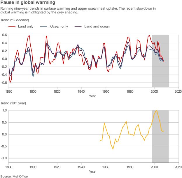
– The lack of a significant increase in the rate of warming during the last century. If we had actually increased the committed warming significantly, the rate of warming should have increased proportionally, but that is not what has been observed (figure 17).
Figure 17. Measure of the rate of warming. Despite a great increase in the amount of CO2 released by humankind to the atmosphere since the 1950s, the rate of warming does not show much of an increase for the past 120 years. This is quite strong evidence that there cannot be a lot of committed warming accumulating every year for the past seven decades, as its cumulative effect is not noticeable in the rate of warming. Source: UK Met Office through the BBC.
– The existence of long periods (decades) with little or no warming should be highly unlikely if we had actually accumulated a huge amount of committed warming.
The only reasonable way to reconcile the disparity in CO2 increases and temperature increases between glacial termination I and the current warming is to conclude that CO2 had a minor role in glacial termination. Further, it is reasonable to expect it will have a minor role in the next glacial inception. The greenhouse theory of paleoclimatology suffers an important blow, along with our confidence that high CO2 levels can protect humankind from glacial inception.
Conclusions
1) Obliquity is the main factor driving the glacial-interglacial cycle. Precession, eccentricity and 65°N summer insolation play a secondary role. There is no 100 kyr cycle. Milankovitch Theory is incorrect.
2) The current pacing of interglacial periods is the consequence of the Earth being in a very cold state that prevents almost half of obliquity cycles from successfully emerging from glacial conditions. The rate for the past million years has been 72.7 kyr/interglacial, or 1.8 obliquity cycles between interglacials. This can be generally described as one interglacial every two obliquity cycles except when close to the 413 kyr eccentricity peaks, when interglacials take place at every obliquity cycle.
3) Glacial terminations require, in addition to rising obliquity, the existence of very strong feedback factors manifested as very low glacial maximum temperatures. High northern summer insolation at the second half of the rising obliquity period is a positive factor, and if high enough during eccentricity peaks can drive the termination process.
4) CO2 can only produce a minor effect in glacial terminations since the measured change in concentration (roughly a third of a doubling which represents half of the warming effect of a doubling) is too small to account for any important contribution to the large observed temperature changes.
5) Since the precession cycle has bottomed and the obliquity cycle is half way down we should expect the next glacial inception to take place within the next two millennia.
Acknowledgements. I thank Andy May for reading the manuscript and improving its English, and Euan Mearns for providing a figure from a publication in press that was the basis for figure 5.
Bibliography. Link to [references].
Methods and Data. Link to [methods-data]
Moderation note: As with all guest posts, please keep your comments civil and relevant.Filed under: Attribution