by Donald C. Morton
The coincidence of the current plateau in global surface temperatures with the continuing rise in the atmospheric concentration of carbon dioxide has raised many questions about the climate models and their forecasts of serious anthropogenic global warming.
This article presents multiple reasons why any future increase in temperature should not be regarded as a vindication of the current models and their predictions. Indefinite time scales, natural contributions, many adjustable parameters, uncertain response to CO2, averaging of model outputs, non linearity, chaos and the absence of successful predictions are all reasons to continue to challenge the present models. This essay concludes with some suggestions for useful immediate actions during this time of uncertainty.
1. Introduction
What if the global climate began to warm again? Would all the criticisms of the climate models be nullified and the dire predictions based on them be confirmed? No one knows when the present plateau in the mean surface air temperature will end nor whether the change will be warmer or cooler. This essay will argue that the climate models and their predictions should not be trusted regardless of the direction of future temperatures.
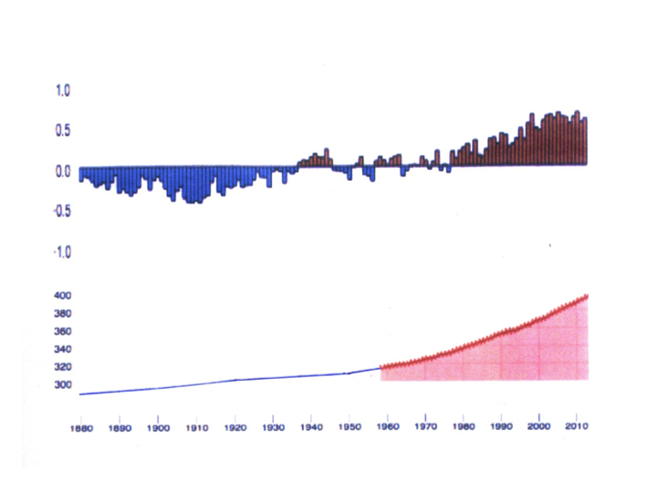
Global temperatures usually are described in terms of the surface air temperature anomaly, the deviation of the temperature at each site from a mean of many years that is averaged over the whole world, both land and oceans. The plots in Fig 1 show how this average has changed since 1880 while the concentration of carbon dioxide (CO2) has steadily increased. The temperature rise from 1978 to 1998 has stopped, contrary to expectations, as shown in Fig. 2 from the latest report of the Intergovernmental Panel on Climate Change (IPCC 2013). Some climatologists like to claim this discrepancy is not sufficient to invalidate their theories and models, but the recent proliferation of papers trying to explain it demonstrates this plateau is a serious challenge to the claims of global disaster.
In this essay I will refer to the present leveling of the global temperature as a plateau rather than a pause or hiatus because the latter two imply we know temperatures will rise again soon. Also I prefer to describe CO2, methane (CH4,), nitrous oxide (N2O), ozone (O3), and the chlorofluoro carbons (CFC’s) as minor absorbing gases rather than greenhouse gases because glass houses become hot mainly by keeping the heated air from mixing with cooler air outside rather than by absorption in the glass. Atmospheric absorption by these gases definitely does warm the earth. The controversy is about how important they are compared with natural causes. We must remember the effect of CO2 is proportional to the logarithm of the concentration while CH4 and N2O contribute according to the square root of concentration but are less abundant by factors of 200 and 1200 respectively. The CFC’s act linearly but the ones still increasing have less than a millionth the abundance of CO2.
IPCC (2013) prefers the term projections rather than predictions for future changes in temperature, but everyone who wishes to emphasize alarming consequences treats the projections as predictions so I will do so here.
Fig. 1. Global Average Temperature Anomaly (°C) (upper), and CO2 concentration (ppm) on Mauna Loa (lower) from http://www.climate.gov/maps-data by the U.S. National Oceanic and Atmospheric Administration. The CO2 curve is extended with ice-core data from the Antarctic Law Dome showing a gradual increase from 291 ppm in 1880 to 334 ppm in 1978. See ftp://ftp.ncdc.noaa.gov/pub/data/paleo/icecore/antarctica/law/law_co2.t….
Skeptics have used this continuing plateau to question whether CO2 is the primary driver of climate, so if temperatures begin to rise again, we can expect many claims of vindication by those who have concluded human activity dominates. An increase is possible as we continue adding CO2 and similar absorbing gases to the atmosphere while natural variability or a continuing decrease in solar activity might result in lower temperatures. It is a puzzle to know exactly what physical processes are maintaining such a remarkable balance among all the contributing effects since the beginning of the 21st century.
Here then are some reasons to continue to distrust the predictions of climate models regardless of what happens to global temperatures.
2. Time Scales
How long do we need to wait to separate a climate change from the usual variability of weather from year to year? The gradual rise in the global surface temperature from 1978 to 1998 appeared to confirm the statement in IPCC2007 p. 10 that, “Most of the observed increase in global average temperatures since the mid-20th century is very likely due to the observed increase in anthropogenic greenhouse gas concentrations”. Then in 2009 when the temperature plateau became too obvious to ignore, Knight et al. (2009), in a report on climate by the American Meteorological Society, asked the rhetorical question “Do global temperature trends over the last decade falsify climate predictions?” Their response was “Near-zero and even negative trends are common for intervals of a decade or less in the simulations, due to the model’s internal climate variability. The simulations rule out (at the 95% level) zero trends for intervals of 15 yr or more, suggesting that an observed absence of warming of this duration is needed to create a discrepancy with the expected present-day warming rate.”
Fig. 2. Model Predictions and Temperature Observations from IPCC (2013 Fig. 11.9). Beginning in 2006, RCP 4.5 (Representative Concentration Pathway 4.5) labels a set of models for a modest rise in anthropogenic greenhouse gases corresponding to an increase of 4.5 Wm-2 (1.3%) in total solar irradiance.
As the plateau continued climatologists extended the time scale. Santer et al. (2011) concluded that at least 17 years are required to identify human contributions. Whether one begins counting in 1998 or waits until 2001 because of a strong El Niño peak in 1998, the 15- and 17-year criteria are no longer useful. To identify extreme events that could be attributed to climate change in a locality, the World Meteorological Organization has adopted a 30-year interval (https://www.wmo.int/pages/themes/climate/climate_variability_extremes.php) while the American Meteorological Society defines Climate Change as “Any systematic change in the long-term statistics of climate elements (such as temperature, pressure or winds) sustained over several decades or longer” (http://glossary.ametsoc.org/wiki/Statistics). Now Solomon, as reported by Tollefson (2014), is saying that 50 to 100 years are needed to recognize a change in climate.
The temperature curve in Fig. 1 does have a net increase from 1880 to 2014, but if we are free to choose both the start date and the interval, wide ranges of slopes and differences are possible so any comparison with climate models becomes rather subjective. If we do not understand the time scale, even if it differs from place to place, we cannot distinguish between the natural variations in weather and a climate change in which we want to identify the human component.
3. Natural Versus Anthropogenic Contributions to Climate Change
Among the multitude of explanations for the temperature plateau there are many that are based on natural causes not fully incorporated in the models. These effects include
- a decreasing concentration of stratospheric water vapor that slowed the rise in surface temperatures (Solomon et al. 2010),
- decadal climate variability (IPCC2013 SPM-10),
- uncertainties in the contributions of clouds (IPCC 2013 9-3; McLean 2014),
- the effects of other liquid and solid aerosols (IPCC 2013 8-4),
- El Niño warming and La Niña cooling in the South Pacific Ocean (de Freitas and McLean, 2013 and references therein; Kosaka and Xie, 2013),
- a multidecadal a deep ocean sink for the missing heat (Trenberth and Fasullo, 2013; Chen and Tung, 2014),
- the Atlantic multidecadal oscillation (Tung and Zhou, 2013),
- a multidecadal climate signal with many inputs propagating across the Northern Hemisphere like a stadium wave (Kravtsov et al. 2014),
- SO2 aerosols from moderate volcanic eruptions (Neely et al., 2013, Santer et al., 2014),
- a decrease in solar activity (Stauning 2014), and
- aerosols in pine forests (Ehn et al. 2014).
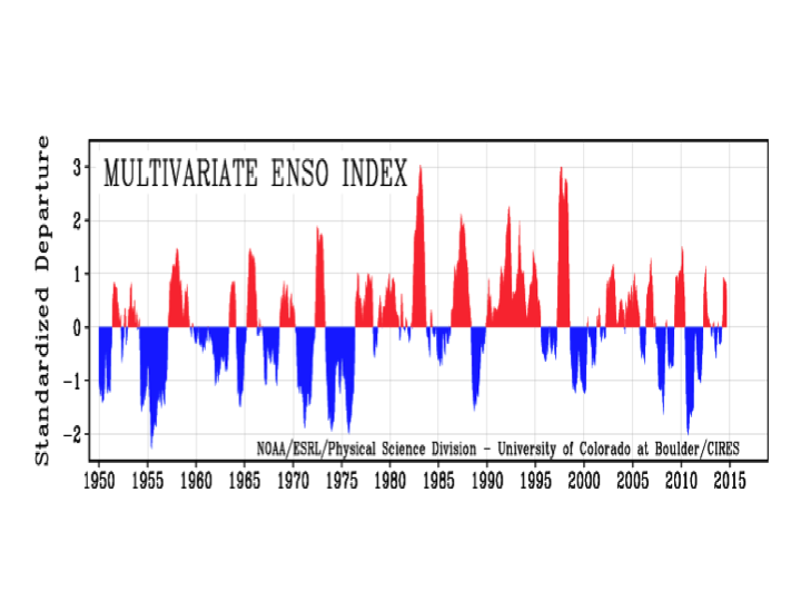
Also, as proposed by Lu (2013) and Estrada et al. (2013), there could be an indirect human effect of reduced absorption by CFC’s resulting from the Montreal Protocol constraining their use. It is not the purpose of this essay to discuss the merits of specific hypotheses, but rather to list them as evidence of incompleteness in the present models. For example Fig. 3 shows the dominance of El Niña warming events from 1978 to 1998 that could account for some of the temperature increase after 1978 as well as the 1998 spike.
When the rising temperatures of the 1980’s coincided with an increasing concentration of CO2, the model makers assumed that human activity was the primary cause, never thoroughly investigating natural contributions. The next step is to assess which ones are significant and add them to the models. Climate predictions without accounting for the relative importance of natural and human effects are useless because we cannot tell whether any proposed change in human activity will have a noticeable effect.
Fig. 3. Multivariate index for the El Niño Southern Oscillation in the Pacific Ocean from the U. S. National Oceanic and Atmospheric Administration. The index combines sea surface air pressure, the components of the surface wind, sea and air surface temperatures and the cloudiness fraction. The upward-pointing red areas indicate El Niño warming intervals and the downward blue ones La Niña cooling.
4. Parameterization in Place of Physics
One often sees the claim that the climate models are based on solid physical principles. This is true in a broad sense, but there are many phenomena that are too complicated or have too small a scale for direct coding. Instead each General Circulation Model (GCM) presented by the IPCC depends on hundreds of parameters that are adjusted (tuned) to produce a reasonable match to the real world. According to IPCC2013 (9-9), ” The complexity of each process representation is constrained by observations, computational resources, and current knowledge.” The availability of time on supercomputers limits the ranges of parameters and the types of models so subjective choices could have influenced the available selection.
IPCC2013 (9-10) further elaborates the challenges of parameterization stating, “With very few exceptions modeling centres do not routinely describe in detail how they tune their models. Therefore the complete list of observational constraints toward which a particular model is tuned is generally not available.” and “It has been shown for at least one model that the tuning process does not necessarily lead to a single, unique set of parameters for a given model, but that different combinations of parameters can yield equally plausible models.”
Parameters are necessary in complex climate modeling, but they have the risk of producing a false model that happens to fit existing observations but incorrectly predicts future conditions. As noted below in Sect. 9, a model cannot be trusted if it does not make correct predictions of observations not used in determining the parameters.
5. Uncertainty in the Climate Sensitivity
The contribution of CO2 to global temperatures usually is quantified as climate sensitivity, either the Equilibrium Climate Sensitivity (ECS) or the Transient Climate Response (TCR). ECS is the increase in the global annual mean surface temperature caused by an instantaneous doubling of the atmospheric concentration of CO2 relative to the pre-industrial level after the model relaxes to radiative equilibrium, while the TCR is the temperature increase averaged over 20 years centered on the time of doubling at a 1% per year compounded increase. The appropriate perturbation of a climate model can generate these numbers once the parameters are chosen. The TCR is a more useful indicator for predictions over the next century because reaching equilibrium can take a few hundred years.
IPCC2013 Table 9.5 quotes a mean TCR = 1.8º (1.2º-2.4º) C and ECS = 3.2º (1.9º-4.5º) C with 90% confidence intervals for a selection of models. This ECS is close to the most likely value of 3º and range of 2.0º to 4.5º adopted in IPCC2007 SPM-12, while IPCC2013 SPM-11 widened the range to 1.5º to 4.5º C, presumably in recognition of the temperature plateau. IPCC2013 SPM-10 admitted there may be “in some models, an overestimate of the response to increasing greenhouse gas and other anthropogenic forcing (dominated by the effects of aerosols)”, but retained the alarming upper limit of 4.5º C from IPCC2007.
Alternative estimates are possible directly from the observed changes in temperature with the increasing concentration of CO2. Huber and Knutti (2012) obtained TCR = 3.6º (1.7º-6.5º 90%) consistent with the models, but others derived lower values. Otto et al. (2012) reported TCR = 1.3º (1.2º-2.4º 95%), ECS = 2.0º (1.2º-3.9º 95%), Lewis and Curry (2014) derived TCR = 1.33º (0.90º-2.50º 95%), ECS = 1.64º (1.05º-4.05º 95%), and Skeie et al. (2014) found TCR = 1.4º (0.79º-2.2º 90%), ECS = 1.8º (0.9º-3.2º 90%). As expected the TCR values always were less than the ECS results.
These wide uncertainties show that we do not yet know how effective CO2 will be in raising global temperatures. If ECS and TCR really are close to the lower end of the quoted ranges, temperatures will continue to increase with CO2 but at a rate we could adapt to without serious economic damage. The recession of 2008 did not have a noticeable affect on the CO2 curve in Fig. 1.
6. Applying Statistics to Biased Samples of Models
Fig. 4 is typical of the IPCC plots of model outputs showing a wide range of possibilities, some of which already represent averages for perturbed parameters of individual models (IPCC 2013 Box 9.1 iii and Sect. 9.2.2.2). Contrary to the basic principles of statistics, the authors of the IPCC Report presumed that the thick red lines representing arithmetic averages have meaning. Averaging is appropriate for an unbiased sample of measurements, not for a selected set of numerical models. Physicists do average the results of Monte-Carlo calculations, but then the inputs must be chosen randomly over the region of interest. This is not so for these climate models because, as noted in Sect. 4, we do not know the selection criteria for most of them. Also, referring to these multimodel ensembles (MME), IPCC (2013 9-17) states, “the sample size of MME’s is small, and is confounded because some climate models have been developed by sharing model components leading to shared biases. Thus, MME members cannot be treated as purely independent.” The following page in the IPCC report continues with “This complexity creates challenges for how best to make quantitative inferences of future climate.”
Fig. 4. In this plot from IPCC (2013 Fig. 9.8), the thin colored lines represent individual models from the Climate Model Intercomparison Project 5 (CMIP5) and the simpler Earth System Models of Intermediate Complexity (EMIC) and the thick red lines their means, while the thick black lines represent three observed temperature sequences. After 2005 the models were extended with the modest RCP 4.5 scenario used in Fig. 2. The horizontal lines at the right-hand side of each graph represent the mean temperature of each model from 1961 to 1990 before all models were shifted to the same mean for the temperature anomaly scale at the left. The vertical dashed lines indicate major volcano eruptions.
Knutti et al (2010) discussed the values of multimodel comparisons and averages and added the cautionary statement, ” Model agreement is often interpreted as increasing the confidence in the newer model. However, there is no obvious way to quantify whether agreement across models and their ability to simulate the present or the past implies skill for predicting the future.” Swanson (2013) provided the example of a possible selection bias in the CMIP5 models due a desire to match the recent arctic warming and remarked that, “Curiously, in going from the CMIP3 to the CMIP5 projects, not only model simulations that are anomalously weak in their climate warming but also those those that are anomalously strong in their warming are suppressed”.
Furthermore the comparisons in Fig. 4 as well as in Fig. 2 attempt to relate the model temperatures to the observations by calculating temperature anomalies for the models without accounting for all the extrapolations of the measurements to cover poorly sampled regions and epochs. Essex, McKitrick and Andresen (2007) have questioned the validity of the global temperature anomaly as an indicator of climate, but since the IPCC continues to compare it with climate models, we should expect agreement. Instead, outside the calibration interval, we see systematic deviations as well as fluctuations in the models that exceed those in the observations.
7. Nonlinearity and Chaos in the Physics of Climate
Climate depends on a multitude of non-linear processes such as the transfer of carbon from the atmosphere to the oceans, the earth and plants, but the models used by the IPCC depend on many simplifying assumptions of linearity between causes and effects in order to make the computation feasible. Rial et al. (2004) have discussed the evidence for nonlinear behavior in the paleoclimate proxies for temperature and in the powerful ocean-atmosphere interactions of the North Atlantic Oscillation, the Pacific Decadal Oscillation and the El Niño Southern Oscillation in Fig. 3.
Frigg et al. (2013) have described some of the approximations in the GCM and their application to derivative models for regional prediction and concluded that “Since the relevant climate models are nonlinear, it follows that even if the model assumptions were close to the truth this would not automatically warrant trust in the model outputs. In fact, the outputs for relevant lead times 50 years from now could still be seriously misleading.” Linearity can be a useful approximation for short-term effects when changes are small as in some weather forecasting, but certainly not for the long-term predictions from climate models.
When the development of a physical system changes radically with small changes in the initial conditions it is classed as chaotic. Weather systems involving convection and turbulence are good examples resulting in computer forecasts becoming unreliable after a week or two. It was an early attempt to model weather that led the meteorologist Edward Lorenz (1963) to develop the theory of chaos. The IPCC Report (2013 1-25) recognizes the problem with the statement “There are fundamental limits to just how precisely annual temperatures can be projected, because of the chaotic nature of the climate system.” However, there is no indication of how long the models are valid even though predictions often are shown to the year 2100.
The difficulties with non-linear chaotic systems are especially serious because of the inevitable structural errors in the models due to the necessary approximations and incomplete representations of physical processes. Frigg et al. (2014) have described how a non-linear model even with small deviations from the desired dynamics can produce false probabilistic predictions.
8. The Validation of Climate Models
How do we know that the models representing global or regional climate are sufficiently reliable for predictions of future conditions? First they must reproduce existing observations, a test current models are failing as the global temperatures remain nearly constant. Initiatives such as the Coupled Model Intercomparison Project 5 (CMIP5) can be useful but do not test basic assumptions such as linearity and feedback common to most models. Matching available past and present observations is a necessary condition, but never can validate a model because incorrect assumptions also could fit past data, particularly when there are many adjustable parameters. One incorrect parameter could compensate for another incorrect one.
The essential test of any physical theory is to make predictions of observations not used in developing the theory. (Of course success in future predictions never is sufficient in the mathematical sense.) In the complicated case of atmospheric models, it is imperative to predict future observations because all past data could subtly influence the permitted ranges of parameters. Unfortunately this test will take the time needed to improve the models, make new predictions, and then wait to see what the climate actually does. Fyfe et al. (2013) aptly described the situation at the end of their paper. “Ultimately the causes of this inconsistency will only be understood after careful comparison of simulated internal climate variability and climate model forcings with observations from the past two decades, and by waiting to see how global temperature responds over the coming decades.”
Through the inadequate inclusion of natural contributions, we lost the recent decades for comparing predictions with observations. It is time for a new start.
9. What Should We Do Now?
Whether global temperatures rise or fall during the next decade or two, we will have no confidence in the predictions of climate models. Should we wait, doing nothing to constrain our production of CO2 and similar gases while risking serious future consequences? If the climate sensitivity to CO2 is near the lower edge of the estimates, the temperature rise could be manageable. Even so many people would argue for major investments to reduce our carbon footprints as insurance. However, as in all situations of risk, we can purchase too much insurance leaving no resources to cope for unforseen developments in climate or other environmental problems. Instead, until there is a new rise in the temperature curve, we have time to pause and assess which projects can be useful and which may be ineffective or even harmful. Here are some proposals.
1) Return to rational discussion, listening to challenges to our favorite ideas and revising or abandoning them as needed, realizing that is how science progresses.
2) Discuss what are optimum global temperatures and CO2 concentrations before we set limits because cold weather causes more fatalities than hot weather and there is evidence that the present warm climate and enhanced CO2 are contributing to increased plant growth (Bigelow et al. 2014).
3) Consider a topic often avoided – the effect of increasing population on the production of CO2 and general sustainability.
4) Cancel subsidies and tax benefits for biofuels because corn competes with food production in temperate zones and palm trees reduce jungle habitat in the tropics.
5) Increase the use of nuclear power, which produces no CO2.
6) Stop asserting that carbon emissions by the industrialized countries are the primary cause of previous warming or sea level rise because undeveloped countries are claiming reparations on this unvalidated premise. (United Nations Climate Change Conference, Warsaw, Poland, 2013 Nov. 11-23).
7) Cease claiming that rising temperatures are causing more occurances of extreme weather because the evidence is not there. (Pielke 2014).
8) Admit that we do not yet understand our climate well enough to say that the science of global warming is settled.
At this stage in the development of the climate models used by the IPCC, it is unclear whether they ever will be useful predictors because the extra computing power needed to reduce the grid scale and time steps in order to adequately include more of the processes that determine weather and climate. There has been no improvement since the ECS estimate of 1.5º to 4.5º C in IPCC (1990 Sect.5.2.1) in spite of an exponential increase in computer capabilities in 23 years. Curry (2014) has emphasized the need to investigate alternatives to the deterministic GCM’s. Including the stochastic nature of climate would be an important next step.
The present temperature plateau has been helpful in identifying the need to consider natural contributions to a changing climate, but the basic problems with the models have been present since their beginning. Whether or not the plateau continues, the current models used by the IPCC are unreliable for predicting future climate.
References [link]
Biosketch. Donald Morton has a Ph.D. in Astrophysics from Princeton, and served as the Director General of the Herzberg Institute for Astrophysics of the National Research Council of Canada. His web page with cv and list of publications is found here [link]. During more than 60 years, his research has followed a variety of topics including spectroscopic binaries, stellar structure, mass transfer in binaries, stellar atmospheres, the interstellar medium, UV spectra from space, QSO spectra, instrumentation for space and ground-based telescopes, observatory management, and the compilation of atomic and molecular data. Now as a researcher emeritus his current interests are theoretical atomic physics, solar physics and astronomical contributions to climate change.
JC note: As with all guest posts, keep your comments relevant and civil.Filed under: climate models