by Javier
Summary: Modern Global Warming has been taking place for the past 300 years. It is the last of several multi-century warming periods that have happened during the Neoglacial cooling of the past 3000 years. Analysis of Holocene climate cycles shows that the period 1600-2100 AD should be a period of warming. The evidence suggests that Modern Global Warming is within Holocene variability, but the cryosphere displays a non-cyclical retreat that appears to have undone thousands of years of Neoglacial ice advance. The last 70 out of 300 years of Modern Global Warming are characterized by human-caused, extremely unusual, rapidly increasing CO2 levels. In stark contrast with this rapidly accelerating anthropogenic forcing, global temperature and sea level appear to have continued their rising trend with no perceptible evidence of added acceleration. The evidence supports a higher sensitivity to CO2 in the cryosphere, suggesting a negative feedback by H2O, that prevents CO2 from having the same effect elsewhere.
Introduction
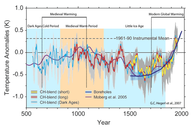
Modern Global Warming (MGW) is the change in climate that has been taking place from the coldest period of the Little Ice Age (LIA) to the present. It is characterized by a preponderance of warming periods over cooling periods, resulting in the warming of the planet, expansion of tropical areas, cryosphere contraction, sea level rise, and a change in dominant weather and precipitation patterns. The nadir of the LIA appears to have been the late Maunder Minimum period of 1660-1715 (Luterbacher, 2001; figure 103). Afterwards, most of the eighteen century was warmer, but was followed by an intense cold relapse in 1790-1820, before the LIA finally ended around 1840. The LIA is the closest the planet has been in 12,000 years to returning to glacial conditions. All over the world most glaciers reached their maximum Holocene extent in the LIA (Solomina et al., 2015; figure 43). But for the past 300 years, MGW has interrupted the Neoglacial cooling trend of the last five millennia. The last 70 years of MGW (25%) has seen considerable, and increasing, human-caused emissions of greenhouse gases (GHG). There is great concern than this and other human actions (deforestation, cattle raising, and changes in land use) might have an important impact over climate, precipitating an abrupt climate change. To some authors the abrupt climate change is already taking place.
Figure 103. Climate variability over the past 1500 years. Proxy reconstruction of 30°-90°N mean annual decadally averaged temperatures over land back to A.D. 558. The time series is made from three segments covered by different amounts of data, which are kept constant within that segment. Gray shaded ranges give the 95% uncertainty bounds of decadal temperature estimates. Moberg et al., 2005, proxy reconstruction and the borehole reconstruction over the same spatial domain are shown for comparison. Each time series is plotted relative to its 1880-1960 mean. Source: G.C. Hegerl et al. 2007. J. Clim. 20, 4, 650-666. Instrumental temperature removed. Main climatic periods are indicated by background color. Multi-centennial warming periods are indicated by horizontal continuous lines and vertical dotted lines.
This series of articles has reviewed how the climate has been changing for the past 800,000 years, and with greater detail for the past 12,000 years. Climate change is the norm, and climate has never been stable for long. It is within this context of past climate change that MGW must be evaluated.
Modern Global Warming is consistent with Holocene climatic cycles
It is often said that MGW is unusual because it contradicts a Neoglacial cooling trend that has been ongoing for several millennia. However, this is a superficial observation. Several multi-centennial warming periods have taken place within the Neoglacial cooling trend. A warming period took place between 1250-850 yr BP (700-1100 AD), leading to the Medieval Warm Period (MWP; Hegerl et al., 2007; figure 103), and another one at 2800-2500 yr BP (850-550 BC), leading to the Roman Warm Period (RWP; Drake, 2012).
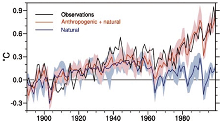
Current models propose that the world would be cooling if it wasn’t for the human influence on climate (Meehl et al., 2004; figure 104).
Figure 104. Models simulate global cooling without anthropogenic forcing. The four-member ensemble mean (red line) and ensemble member range (pink shading) for globally averaged surface air temperature anomalies (°C) for all forcings [(volcano + solar + GHG + sulfate + ozone)]; the solid blue line is the ensemble mean and the light blue shading is the ensemble range for globally averaged temperature response to natural forcings [(volcano + solar)]; the black line is the observations after Folland et al. (2001). Source: G.A. Meehl et al. 2004. J. Clim., 17, 19, 3721-3727.
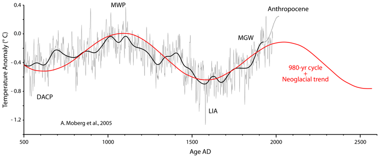
However, the proposition that the world should be cooling absent an anthropogenic effect, contradicts our knowledge of Holocene climate cycles. One of the main cycles is the ~ 1000-year Eddy cycle found in climate and solar activity proxy records of the Early and Late Holocene (see: Centennial to millennial solar cycles). The periodicity of this cycle is maintained from Early to Late Holocene, and reflected in the Bond events of increased iceberg activity in the North Atlantic (figure 81). The start of the Medieval Warming ~ 700 AD, and the start of the MGW at ~ 1700 AD are separated by ~ 1000 years. The peak of the MWP at ~ 1100 AD and the trough of the LIA at ~ 1600 are separated by ~ 500 years (figure 103). Based on this cycle it can be projected that the period ~ 1600-2100 AD should be a period of net warming, to be followed by a cooling period ~ 2100-2600 AD, if the cycle maintains its beat (figure 105).
Figure 105. Warming and cooling periods of the past 1500 years, fitted to known climate cyclic behavior. Moberg et al., 2005, reconstruction of Northern Hemisphere temperature anomaly for the period 500-1978 AD (grey curve), and its low frequency component (black curve). The 980-year Eddy cycle is shown in red, with a declining Neoglacial trend of –0.2 °C/millennium. As Moberg’s reconstruction ends in 1978, the dotted line represents the 1975-2000 warming, that is similar in magnitude to the 1910-1945 warming. DACP, Dark Ages Cold Period. MWP, Medieval Warm Period. LIA, Little Ice Age. MGW, Modern Global Warming. Peak natural warming is expected in 2050-2100 AD.
There might be an anthropogenic contribution in the MGW, but it is clear that warming at this time is not unusual, and in fact, it is about what should be expected. The most logical conclusion is that natural warming is contributing to the observed warming. If models are not capable of simulating this natural warming, of millennial cyclic origin, then the models must be wrong, and our knowledge of climate change insufficient.
Modern Global Warming is within Holocene variability
How unusual is the warming observed during MGW?. This is a very difficult question to answer. Temperature is an intrinsic intensive property that is changing during the course of a day at any point on the surface of the planet in an unpredictable direction and rate. If there is a global average temperature, we have no way of measuring it. However, we have devised methods of measuring temperature (or radiation) at different points on the surface (with huge areas unsampled) or in the atmosphere. A consistent mathematical treatment of this data gives a consistent value that we term average temperature, although it is not a temperature, but a conversion of intrinsic intensive measurements into an extrinsic extensive value using multiple assumptions.
However, the global average temperature concept is useful as the calculated value shows much less change over time than the measured values, and we term that change “anomaly,” wrongly implying that it should be constant over time. The change in the global anomaly over the years shows a correlation to real physical and biological phenomena, like length of the growing season, extent of the cryosphere, and sea level rise, among others, and thus it is useful. However, two dangers should be avoided when dealing with the global temperature anomaly. The first is using the same units for temperature as for the temperature anomaly. The degrees in the temperature anomaly are different than the degrees in temperature, since the connection to physical degrees is lost in the conversion from intrinsic to extrinsic. Many authors are unaware of this problem and attempt to compare proxy derived local temperatures to an instrumental calculated global anomaly. Also, the precision given in a temperature anomaly is not a precision in measurement, but a precision in calculation. This is also important as the real uncertainty cannot be calculated, due to multiple assumptions in the process that are no properly evaluated. Another danger is that averaging changes in temperature ignores differences in enthalpy (internal energy and the product of temperature and pressure or, more simply the “heat content”). Due to its low humidity, especially in winter, big changes in Arctic air temperature can take place with small changes in heat content. The weight that Arctic air temperatures should have in a global average is an unresolved question that is biasing instrumental temperature anomalies, relative to temperature proxies.
So, going back to our problem we are now calculating a global temperature with our chosen method, but with no way to relate it to anything similar from the past. Even our calculated anomaly becomes pure fiction (if it wasn’t already) when moving into the 19th century. The way we estimate climate change from the past is through proxies. The relationship of proxies to temperature is convoluted. Some proxies respond to summer temperature changes, while others to winter or spring temperatures. Other factors, like rate of deposition, rate of upwelling, precipitation, cloud cover, storm frequency, or wind, might affect a proxy often without a clear possibility of correction, as the researcher might be unaware of the bias. The resolution of proxies cannot match the resolution of our measurements. The 2014-16 El Niño that increased our global anomaly by 0.4°C for a short period would not be resolved by most proxies. And proxies are always local in nature. That’s why most serious scientists abstain from attempting to calculate past global temperature averages from collections of proxies, and avoid linking them to modern instrumental temperature anomalies. They are two very different things.
However, we can answer the question of how unusual MGW is. Biology offers us a solution. The treeline represents the limit where climatic conditions allow the establishment of new trees. Every year new tree seedlings attempt to establish themselves further up the mountain and generally fail. 52% of studies show the treeline has been going up for the past century, and only 1% show a line receding, indicating that mountain trees are generally responding to global warming and increased CO2 by raising the treeline (Harsch et al., 2009). However, many studies show that at most places the present treeline is still 100-250 meters below Holocene Climatic Optimum treeline levels (figure 106; Reasoner & Tinner, 2009; Cunill et al., 2012; Pisaric et al., 2003).
Figure 106. Holocene treeline changes in the Alps. The approximate Holocene timberline and treeline elevation (m above sea level) in the Swiss central Alps based on radiocarbon-dated macrofossil and pollen sequences. Source: M.A. Reasoner & W. Tinner. 2009. Encyclopedia of Paleoclimatology and Ancient Environments (pp. 442-446).
We must take into account that present elevated CO2 levels might give current trees an advantage over Early Holocene trees. The difference in treeline altitude between now and the Early Holocene imply that MGW is not unusual enough to have returned us to Holocene Climatic Optimum conditions. Therefore, present global warming is within Holocene variability. Reasoner and Tinner (2009) quantify the summer temperature difference in the Alps between now and the Holocene Optimum as: “Assuming constant lapse rates of 0.7° C / 100 m, it is possible to estimate the range of Holocene temperature oscillations in the Alps to 0.8–1.2° C between 10,500 and 4,000 cal. yBP, when average (summer) temperatures were about 0.8–1.2° C higher than today.”
The cryosphere confirms that present conditions are within Holocene variability, as globally glaciers reached their shortest extent at times between 10,000 and 5,000 years ago, when many glaciers that now exist were absent (Solomina et al., 2015). Arctic sea ice was also very much reduced during the Holocene Climatic Optimum compared to present day, and perhaps ice free (less than 1 million km2) during the summers at some periods (Jakobsson et al., 2010; Stein et al., 2017).
MGW is not unusual by Holocene standards in its amplitude, duration, and timing. We cannot rule out that the magnitude of the warming, while not unusual for the Holocene, is unusual for the Neoglacial period that, after all, is characterized by a multi-millennial downward trend in temperatures. If that is the case however it is very difficult to demonstrate because of the mentioned problems of comparing present and past temperatures. Circumstantial evidence supports that the RWP was warmer than present (Holzhauser et al., 2005), but the RWP was extraordinarily long, a millennium, so some of its effects might be because of the long time spent in a warm state not necessarily warmer than the present.
Modern Global Warming displays an unusual cryosphere response
If MGW is not unusual by Holocene standards, it becomes important to inquire about the climatic response to the increased atmospheric CO2 levels. Is there anything unusual about MGW? The answer is a clear yes. The cryosphere (with the exception of Antarctica) is showing a very unusual response to MGW. For the last two decades glaciologists have recognized that global glacier changes over the past 170 years are not cyclical and greatly exceed the range of the previously known periodic variations of glaciers (Solomina et al., 2008; figure 107). Koch et al. (2014), attest that the global scope and magnitude of glacier retreat likely exceed the natural variability of the climate system and cannot be explained by natural forcing alone. Goehring (2012) states that after 5 kyr BP, the Rhône Glacier was larger than today, and its present extent therefore likely represents its smallest since the middle Holocene. Solomina et al. (2008) defend that Alpine glacier volumes have become smaller now than during at least the past ~ 5000 years. And Bakke et al. (2008; figure 107 d) have measured a retreat of maritime glaciers along western Scandinavia over the last century that is unprecedented in the entire Neoglacial period spanning the last 5200 years. Solomina et al. (2016) resume the global glacier situation:
“The current globally widespread glacier retreat is unusual in the context of the past two millennia and, indeed, for the whole Holocene. Contemporary glacier retreat breaks a long-term trend of increased glacier activity that dominated the past several millennia. The trend of glacier retreat is global, and the rate of this retreat has increased in the past few decades. The observed widespread glacial retreat in the past 100–150 years requires additional forcing outside the realm of natural changes for their explanation.”
Figure 107. Modern glacier retreat is not cyclical. a) Time-distance diagram for glacier extent on the Central Cumberland Peninsula (Baffin Island) through the Holocene. Source: J.P. Briner et al. 2009. Quat. Sci. Rev. 28, 2075–2087. b) Glacier fluctuations in the Himalaya and Karakoram up to 1980, defined by radiocarbon dating. Source: L.A. Owen. 2009. Quat. Sci. Rev. 28, 2150–2164. c) Relative glacier extent fluctuations in western Canada during the Holocene. Source: J. Koch & J.J. Clague. 2006. PAGES News 14, 3, 20-21. d) Combined equilibrium-line altitude (ELA) variations along the south-north coastal transect in Norway. The glacier growth index is obtained by adding standardized ELA estimates from southern and northern Norway. Source: J. Bakke et al. 2008. Glob. Planet. Change, 60, 1-2, 28-41.
Global glacier retreat is probably the only climate-associated phenomenon that shows a clear acceleration over the past decades. The World Glacier Monitoring Service, an organization participated by 32 countries, holds a dataset of 42,000 glacier front variations since 1600, that show that the rates of early 21st-century glacier mass loss are without precedent on a global scale, at least since 1850 (Zemp et al., 2015).
Unusual glacier retreat is confirmed by the loss of small permanent ice patches, also known as glacierets. These permanent ice patches have captured and preserved archeological organic remains during their long existence, and the remains are now being released as they melt. This is the origin of the new subfield of ‘ice patch’ archeology, that has developed in three regions, North America, the Alps, and Norway. Some plant remains, like tree trunks (figure 108 a & b), or the Quelccaya plants dated at ~ 5200 BP (Thompson et al., 2006) are naturally occurring and their burial in ice is related only to climatic conditions, but archeological remains (figure 108 c-f) reflect human activity and are thus more complex. Alpine findings are related to the use of mountain passes when conditions improved, and their dating shows asynchrony with North American findings, associated with summer hunting of caribou, that takes refuge from insects over ice patches. Thus, Alpine findings are more frequent from warm phases and at the beginning of cold phases, while North American findings are more frequent from cold phases when ice patches became more widespread. (figure 108 f). Most organic remains, like leather (figure 108 d), caribou dung, or corpses (Ötzi, dated at ~ 5200 BP, figure 108 c), are not preserved when exposed for even relatively short periods, and it is clear that they have remained continuously frozen since first buried in ice. Their present climate induced unburial is clear evidence that small permanent ice patches are experiencing a reduction not seen since the Mid-Holocene Transition. “The [‘ice patch’ archeology] field is characterized by a sense of urgency about recovering and preserving both those occasional human remains melting from alpine ice and newly-exposed artifacts of rare and fragile organic technology” (Reckin, 2013).
Figure 108. Organic remains recently unburied from ice. a) Detrital wood near the snout of Helm Glacier, exposed by glacier retreat in the summer of 2003. b) In situ stump (top arrow) and stem (bottom arrow), 600 m from the snout of Lava Glacier in 2003. c) Ötzi, the alpine iceman, in situ before his removal from the site at Niederjoch, Italy, in 1991. d) Iron Age leather shoe recovered from Langfonna ice patch, Jotunheimen, Norway, in 2006. e) Artifacts recovered from an alpine ice patch in the Yukon. Source for a)-e): J. Koch et al. 2014. The Holocene, 24, 12, 1639–1648. f) Summed probability of available radiocarbon dates for the Alps (grey line) and North America (black line) ice patch archeological findings. They demonstrate the probability that a date from each collection will fall within a particular period and exclude typologically-dated material (most of which is Roman in age). They have been smoothed to a 200-year interval to remove extraneous noise and emphasize more general trends. Source for f): R. Reckin. 2013. J. World Prehist. 26, 4, 323-385.
Arctic sea ice has displayed a similar behavior to glaciers, with a very pronounced reduction at the turn of the century (1996-2007), losing 30% of its summer extent in just a decade. This reduction is not outside Holocene variability, as multiple studies document a much lower Arctic sea ice extent between 9000 and 4000 BP (Belt et al., 2010; Jakobsson et al., 2010; Stranne et al., 2014; Stein et al., 2017), but appears excessive for just a decade within a multi-centennial cyclic warming period. The difficulty in reconstructing past sea ice levels means that we don’t have much confidence in how the present reduction in sea ice extent compares to previous reductions during past warm periods. However, an analysis of polar ice shelves (thick floating ice platforms), shows an unusual response in present polar ice retreat. Although ice shelves have collapsed and broken up at different times during the Holocene, this is the first time in the Holocene when a synchronous retreat in ice shelves from the Arctic and both sides of the Antarctic Peninsula is known to have occurred (Hodgson, 2011; figure 109).
Figure 109. Polar ice shelves Holocene reconstruction. Presence and absence of polar ice shelves that have broken up or retreated in the past few decades. Solid blue bars show periods when the ice shelves were present, red bars show periods of absence or retreat, and empty bars show where a grounded ice sheet was present. a) Sea ice proxy record from diatom-derived biomarker IP25 in Victoria Strait (Canadian Arctic Archipelago) from Belt et al., 2010. Ward Hunt ice shelf on Ellesmere Island (Canadian Arctic). b) George VI ice shelf, west of the Antarctica Peninsula, and Prince Gustav, and Larsen A and B ice shelves, east of the Antarctic Peninsula. Source: D.A. Hodgson. 2011. PNAS, 108, 47, 18859–18860.
Antarctica is an exception to the global reduction of the cryosphere. The continent hasn’t warmed for the past 200 years (figure 110), and it is currently debated if Antarctic melting is contributing to sea level rise and by how much (Zwally et al., 2015). Antarctic lack of climatic response to MGW and CO2 increase is not well understood, and it might have to do with the exceptional conditions of the continent that make it unique in many aspects.
Extremely unusual CO2 levels during the last quarter of Modern Global Warming
Another stark difference between MGW and previous Holocene warming periods is the great increase in CO2 levels. Atmospheric CO2 has been increasing since ~ 1785, following the 18th century warming, but the rate of increase has been growing continuously due to anthropogenic emissions, reaching the highest values in 800,000 years by the first decades of the 20th century, and it is now fast approaching a doubling of the Late Pleistocene average value of 225 ppm (figure 110). It is absolutely clear that the increase in CO2 levels is due to human emissions, as we have emitted double the amount that has ended up in the atmosphere, the rest being taken up by the oceans and biosphere, that is showing an important increase in global leaf area (Zhu et al., 2016), also known as greening.
The Antarctic Plateau is the only place on Earth where we can measure CO2 levels and proxy temperatures in a consistent manner for the past 800,000 years from ice cores. Much has been written about the close correlation between CO2 and temperatures over the Late Pleistocene (figure 110 a). The change of CO2 levels between glacial and interglacial periods, of only 70–90 ppm, is considered by most authors to be too small to drive the glacial cycle, although Shakun et al., (2012) defend that the CO2 change at terminations can explain a large part of the temperature increase during deglaciations. But we can test the hypothesis because over the last 200 years CO2 levels have increased by 125 ppm, an increase comparable to that of a glacial termination in terms of CO2 forcing. Surprisingly, Antarctica shows absolutely no warming for the past 200 years (Schneider et al., 2006; figure 110 b). The only place where we can measure both past temperatures and past CO2 levels with confidence shows no temperature response to the huge increase in CO2 over for the last two centuries. This evidence supports that CO2 has very little effect over Antarctic temperatures, if any, and it cannot be responsible for the observed correlation over the past 800,000 years. It also raises doubts over the proposed role of CO2 over glacial terminations and during MGW.
Figure 110. Antarctic ice cores temperature–Ln(CO2) discrepancy. a) Temperature curve (blue) for the past 800,000 years from EPICA Dome C Ice Core 800KYr Deuterium Data. Source: NOAA, contributed by Jouzel et al., 2007. CO2 curve (red) from Antarctic Ice Cores Revised 800KYr CO2 Data (to 2001). Source: NOAA, contributed by Bereiter et al., 2015; and from NOAA annual mean CO2 data (2002–2017). Due to the logarithmic effect of CO2 on temperatures, the comparison is more appropriately done with the Ln(CO2). The correlation shows a very big discrepancy over the last 200 years. b) CO2 curve (red) as in a). Temperature curve (blue) for the past 200 years from 5 high resolution Antarctic ice cores. Source: D.P. Schneider et al. 2006. Geophys. Res. Let. 33, L16707. No temperature change is observed in response to the massive increase in CO2.
The relationship between CO2 levels and temperature during Modern Global Warming
Physics shows that adding carbon dioxide leads to warming under laboratory conditions. It is generally assumed that a doubling of CO2 should produce a direct forcing of 3.7 W/m2 (IPCC-TAR, 2001), that translates to a warming of 1°C (by differentiating the Stefan-Boltzmann equation) to 1.2°C (by models taking into account latitude and season). But that is a maximum value valid only if total energy outflow is the same as radiative outflow. As there is also conduction, convection, and evaporation, the final warming without feedbacks is probably less. Then we have the problem of feedbacks, which are unknown and can’t be properly measured. For some of the feedbacks, like cloud cover we don’t even know the sign of their contribution. And they are huge, a 1% change in albedo has a radiative effect of 3.4 W/m2 (Farmer & Cook, 2013), almost equivalent to a full doubling of CO2. So, we cannot measure how much the Earth has warmed in response to the increase in CO2 for the past 70 years, and how much for other causes.
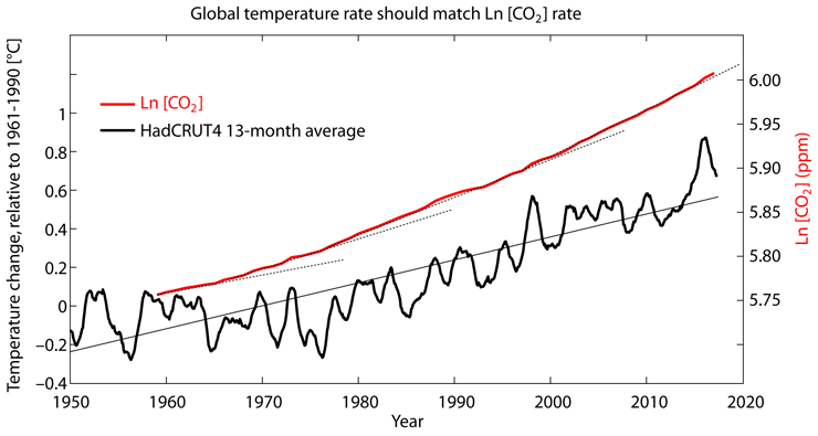
Looking at borehole records and proxy reconstructions (figure 103), it becomes very clear that most of the acceleration in the rate of MGW took place between 1700 and 1900, when very little human-caused GHGs were produced. The rate of warming has changed little in the 20th and 21st centuries, despite the bulk of GHGs being emitted in these past 70 years. However, if the increase in global average temperature over the past 7 decades was mainly a consequence of the rapid increase in CO2, the rate of temperature change should show dependence on the rate of change of the natural logarithm of CO2 concentration. This is because the proposed link between CO2 and temperature is based on a molecular mechanism where every added molecule has slightly less effect than the previous. Even accounting for the logarithmic response of global average temperatures to CO2, the curves for proposed cause and effect are clearly diverging (figure 111). The global temperature anomaly between 1950 and 2017 is not significantly different from a linear trend. On the other hand, atmospheric CO2 increase has been so fast over the 1958-2017 period that the rate of change of its logarithm displays a pronounced acceleration (figure 111).
Figure 111. The difference between temperature increase and CO2 increase. Thick black curve, HadCRUT4 13-month centered moving average surface temperature anomaly, relative to 1961-1990, from 1950 to 2017 (November). Source: UK Met Office. The thin continuous line is a linear trendline of the temperature data. Thick red curve, the natural logarithm of the 1958-2017 annual atmospheric CO2 concentration (ppm). Source: NOAA. Thin black dotted lines, visual aid showing the effect of the rapid increase in CO2 concentration on its logarithm. It is proposed that the increase in the logarithm of CO2 is causing the increase in temperature, yet the curves diverge.
The lack of MGW acceleration during the 20th-21st centuries can be more readily appreciated when looking at the change in warming rate (decadal trend change; figure 112). Over that period the warming rate has been oscillating between –0.2 and +0.4 °C/decade with an average of +0.16 °C/decade. Neither the warming rate maximum, nor the length of the warming periods have increased despite the huge increase in CO2 levels. The expected warming effect of the additional CO2 is not perceptible in warming rates. What can be seen in the warming rate record is that cooling periods have become less intense, from –0.4 °C/decade in the late 19th century, to –0.2 °C/decade in the mid-20th century, to zero in the 21st century pause. This decrease in cooling rate over time is a feature of MGW. The world is warming because it cools less during cooling periods, not because it warms more during warming periods. The reasons for this are unclear, and not discussed often in the scientific literature. There is a coincidental reduction in periods of very low solar activity, that also usually coincide with cooling periods, but other factors cannot be ruled out, including an effect from increased CO2 levels at reducing the severity of cooling periods, or a reduction in volcanic activity.
Figure 112. Surface warming trend. Running nine-year trends in surface warming. Red line, land only. Blue line, ocean only. Black line, land and ocean combined. Source: UK Met Office 2013, through the BBC.
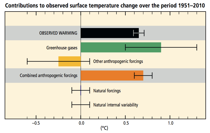
The lack of MGW acceleration despite the rapid increase in CO2 over the past 7 decades only has two possible explanations. The first is that the ongoing increase in the proposed anthropogenic forcing exactly matches in magnitude and time an ongoing decrease in natural forcing (figure 104). The second is that MGW responds more to natural causes, and only weakly to anthropogenic forcing. The first explanation constitutes an “ad hoc” match of hypothesis to evidence, requires an unrelated coincidence of decadal precision within a multi-century process (natural cooling started just when we started our emissions), and it is disavowed by the IPCC, that considers natural forcing over the 1950-2010 period too small to have contributed to the observed temperature change in any direction (figure 113). That natural forcing has had no role over a 60-year period is hard to believe.
Figure 113. IPCC proposed contributions to observed surface temperature change over the period 1951-2010. IPCC assessed likely ranges (whiskers) and their mid-points (bars) for warming trends over the 1951–2010 period from well-mixed greenhouse gases, other anthropogenic forcings (including the cooling effect of aerosols and the effect of land use change), combined anthropogenic forcings, natural forcings and natural internal climate variability. The observed surface temperature change is shown in black, with the 5 to 95% uncertainty range due to observational uncertainty. The attributed warming ranges (colours) are based on observations combined with climate model simulations, in order to estimate the contribution of individual external forcings to observed warming. Source: IPCC. 2014. AR5. Synthesis Report. Summary for policymakers. Figure SPM.3 p. 6.
The second explanation requires only an insufficient knowledge of the response of the climatic system to CO2, and an insufficient knowledge of natural forcings and climate feedbacks. That our knowledge is insufficient is clear and demonstrated every time the “argumentum ad ignorantiam” that “we don’t know of anything else that could cause the observed warming” is used. New research into solar variability mechanisms (see: Climate change mechanisms) has produced hypotheses that indicate that solar forcing is probably not adequately represented in models, and the cloud feedback is essentially not understood yet.
Uniform variation in sea level during Modern Global Warming
Sea level rise (SLR), is one of the main consequences of MGW as it is driven mainly by the addition of water from melting of the cryosphere, and thermal expansion of the warming oceans (steric SLR).
A recent sea level reconstruction since the 18th century using tide gauge records (Jevrejeva et al., 2008; figure 114 a) shows that sea level rise has been a feature of MGW for over two centuries. The central estimate on 20th-century average SLR is ~ 1.6 mm/yr (1.2-1.9 mm/yr range), and the acceleration is usually estimated at ~ 0.01 mm/yr2 (Church & White, 2011; Jevrejeva et al., 2014; Hogarth, 2014; figure 114 b). SLR displays a 60-year oscillation, like many other climatic manifestations (see: Climate change mechanisms). The recent period of satellite altimetry (1993-2017) coincides with the crest of the oscillation, and thus shows a higher rate of SLR, ~ 3.0 mm/yr, but no acceleration, to the surprise of some authors (Fasullo et al., 2016). If the 60-year oscillation continues affecting SLR, over the next couple of decades we should expect a deceleration of SLR rates towards ~ 2 mm/yr.
Figure 114. Sea level acceleration started over 200 years ago. a) Time series of yearly global sea level calculated from 1023 tide gauge records corrected for local datum changes and glacial isostatic adjustment. Time variable trend detected by Monte-Carlo-Singular Spectrum Analysis with 30-year windows. Grey shading represents the standard errors. b) The evolution of the rate of the trend (black line) showing multidecadal variability. Blue line corresponds to the linear background sea level acceleration that corresponds to a sea level acceleration of 0.01 mm/yr2. Red line, IPCC calculated total anthropogenic radiative forcing. Source: S. Jevrejeva et al. 2008. Geophys. Res. Let. 35, L08715. IPCC AR5. 2013.
As was the case with temperature, SLR precedes the big increase in emissions, and does not respond perceptibly to anthropogenic forcing. Figure 114 b displays the linearly adjusted trend in long term average SLR acceleration as a blue line, and the increase in anthropogenic forcing (IPCC-AR5, 2013) with a red line. The evidence shows that the big increase in anthropogenic forcing, has not provoked any perceptible effect on SLR acceleration. The belief that a decrease in our emissions should affect the rate of SLR has no basis in the evidence. A projection of the observed SLR and acceleration for the past 120 years gives a value of ~ 280 mm more in 2100 than in 2017.
Cryosphere melting is considered the main factor driving SLR, followed by ocean temperature increase. However, SLR displays a small acceleration of ~ 0.01 mm/yr2 over the past two centuries (figure 114), while global temperature shows a linear increase over the past century, and the ocean is warming a lot less than the surface. It has been recently estimated from changes in atmospheric noble gases, that the ocean has warmed +0.1 °C for the past 50 years (Bereiter et al., 2018, see the press release). The best candidate for causing the observed SLR acceleration is therefore the observed increase in cryosphere melting since ~ 1850.
Modern Global Warming and the CO2 hypothesis
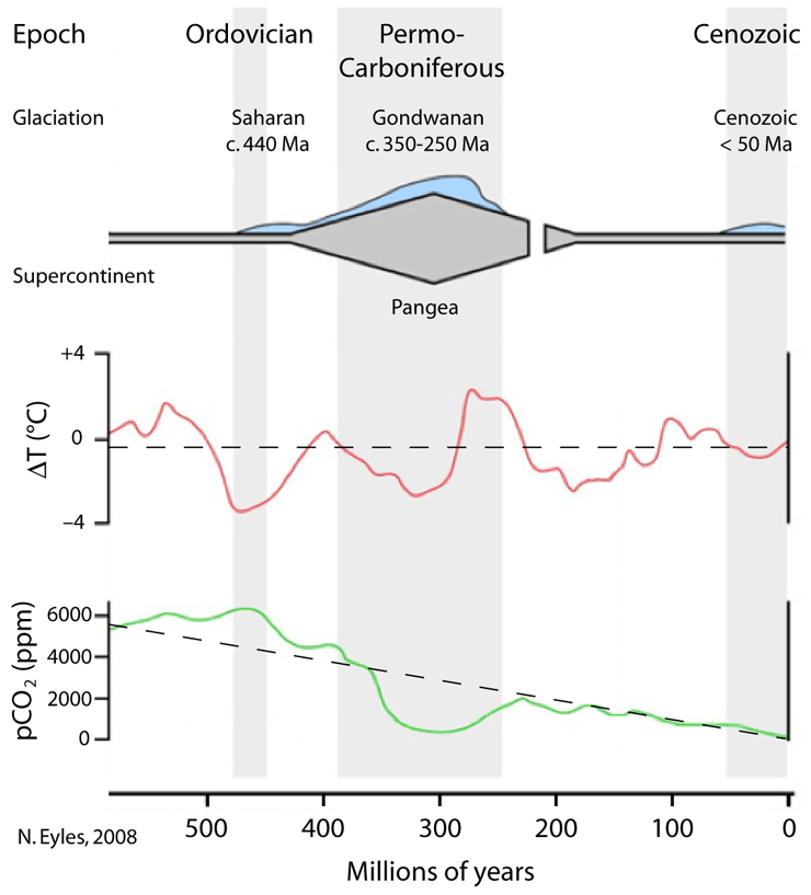
The CO2 hypothesis proposes that changes in atmospheric CO2 levels are the main driver of Earth temperature changes (Lacis et al., 2010). It is based on the spectral absorption and radiation properties of certain gases, of which water vapor is by far the most abundant, and CO2 is a distant second. Water vapor levels are locally determined and highly variable due to condensation. CO2 levels are global, as it is a well-mixed gas that does not condense, and before industrialization it changed very slowly over time from natural causes. CO2 hypothesis considers that water vapor changes are not the driving factor, but a feedback, proposing without clear evidence that the relevant causal relationship is CO2 –> temperature –> water vapor. Past water vapor levels cannot be determined, but in the distant past, cold periods of the planet (Ice Ages) were associated to lower CO2 levels than warm periods, and this is the supporting evidence offered by proponents of the CO2 hypothesis. The interpretation of this evidence, however, is far from straightforward, as changes in temperature also lead to changes in CO2, from huge ocean carbon dioxide stores, because the gas solubility is dependent on temperature, and in well resolved records, changes in temperature generally precede changes in CO2 by hundreds to thousands of years. Another problem with the hypothesis is that it is generally accepted that a progressive decrease in CO2 levels has taken place for the past 550 million years (the Phanerozoic Eon), from ~ 5000 ppm in the Cambrian to ~ 225 ppm in the Late Pleistocene. This decrease does not appear to have produced a progressive decrease in temperatures, that display a cyclical range-bound oscillation (Eyles, 2008; figure 115), alternating between icehouse and hothouse conditions over the entire Phanerozoic.
Figure 115. Phanerozoic Eon conditions don’t support the CO2 hypothesis. Schematic representation of glacio-epochs during the past 550 million years in Earth history, and their relationship to phases of supercontinent assembly and break up. Glaciations are indicated and represented by the blue area above the scheme. Estimated global temperature trends (red graph), and variations in atmospheric carbon dioxide (green graph), are indicated, with their general trend as a dashed line. Surce: N. Eyles. 2008. Palaeo3 258, 89–129.
The CO2 hypothesis is not new, and can be traced to Arrhenius in 1896, however it did not become the dominant hypothesis to explain temperature changes until the last warming phase of MGW started in the late 1970’s, and temperature and CO2 were both increasing.
In the 20th century, while MGW was taking place, humanity embarked in the ultimate experiment to determine the validity of the CO2 hypothesis and set about to burn huge fossil fuel natural stores while industrializing, to raise CO2 levels beyond what the world has had in perhaps millions of years. After 70 years with CO2 levels increasing faster than ever recorded, and above any previously recorded level for the Late Pleistocene, it is time to analyze the results.
- The world has continued warming as before. The warming during the 1975-1998 (or 1975-2009) period is not statistically significantly different from the warming during the 1910-1940 period (Jones, 2010).
- The temperature increase since 1950 shows no discernible acceleration and can be fitted to a linear increase. The logarithm of the CO2 increase, however, displays a very clear acceleration (figure 111). A linear relation between supposed cause and effect cannot be established.
- Sea level has continued rising as before. Its acceleration is not responding perceptibly to the increase in anthropogenic forcing (figure 114).
- The cryosphere shows a non-cyclical retreat in glacier extent with evidence of acceleration (figure 107; Zemp et al., 2015). The reduction of the size of ice shelves is also unusual (figure 109). The evidence supports a cryosphere response to the CO2 increase.
- Despite CO2 levels that are almost double the Late Pleistocene average, the climatic response is subdued, still within Holocene variability, below the Holocene Climatic Optimum and below warmer interglacials.
Lack of support for the CO2 hypothesis from Antarctic ice cores (figure 110), and from results 1-3 has forced the proponents of the hypothesis to make numerous new unsupported assumptions. They assume that all warming since 1950 is anthropogenic in nature (IPCC-AR5, 2014, figure 113). That past recorded temperatures must be cooler than previously thought (Karl et al., 2015). That the oceans (Chen & Tung, 2014), and volcanic eruptions (Fasullo et al., 2016), are delaying the surface warming and SLR. And essentially concluding that more time is required to observe the warming and SLR acceleration. All these might be true, but the simplest explanation (Occam’s favorite) is that an important part of the warming is due to natural causes, and CO2 only has a weak effect on temperatures. If after 70 years of extremely unusual CO2 levels, a lot more time is required to see substantive effects, then the hypothesis needs to be changed. As proposed it does not call for long delays, due to the near instantaneous effect of the atmospheric response to more CO2. The CO2 hypothesis is at its core an atmospheric-driven hypothesis of climate. There is a significant possibility however that the climate is actually ocean-driven, directly forced by the Sun, and mediated by H2O changes of state.
The high sensitivity of the cryosphere to the CO2 increase might actually be an argument for a reduced sensitivity by the rest of the planet. The air above the cryosphere is the coldest of the planet, as it is not warmed much from below, and therefore it has the lowest humidity of the planet. The ratio of water vapor to CO2 in the air above the cryosphere is the lowest and the one that changes the most with the increase in CO2. There is the possibility that air dryness, and the low capacity to produce water vapor in response to warming might be the reasons why the cryosphere is particularly sensitive to CO2, but it implies the rest of the planet is less sensitive. If CO2 sensitivity is highest over the cryosphere (except Antarctica), and lower over the rest of the planet, this points to a negative feedback by H2O response, in its three states, to temperature changes. Antarctica doesn’t show increased sensitivity because it has not been warming through the entire MGW, regardless of CO2.
There are multiple possible H2O temperature regulatory mechanisms, and the proposition that H2O only acts as a fast-positive feedback to CO2 changes is too simplistic. The huge water mass in Earth’s oceans and its slow mixing, add a great thermal inertia that resists temperature changes. Atmospheric humidity determines how changes in energy translate into changes in temperature, as humid air has a higher heat capacity and responds to the same energy change with a lower temperature change than dry air. Atmospheric humidity responds very fast to temperature changes through evaporation and condensation. This mechanism is proportional to water availability, and works better above the oceans than over land, and very little over the cryosphere, inversely correlating to MGW temperature changes, that are highest in the Arctic (polar amplification), and lower over the oceans than over land. To that we must add other region-specific temperature-regulating mechanisms by H2O. Deep convection is a tropical atmospheric phenomenon that takes place when the surface of the tropical ocean reaches 26-30 °C. The ocean flips from absorbing energy to releasing it, and convection takes the energy very high in the troposphere, cooling the ocean (Sud et al., 1999) and effectively limiting its maximum temperature. Polar sea ice is a negative feedback that releases heat when it forms in the autumn, then absorbs heat, when it melts in spring, and it acts as an insulator preventing ocean heat loss during winter. Ice-albedo effect is a positive feedback, in that a decrease in ice reduces albedo, driving further ice loss. But ice-albedo feedback is ameliorated because ice extent moves opposite to sunlight (maximum ice coincides with minimum albedo when it is darker), and by the high inclination of the Sun’s rays at polar latitudes, making water more reflective. So the albedo effect is not driving Arctic sea ice melting as demonstrated by the 10-year pause in summer Arctic sea ice loss, after losing 30% of its extent the previous 10-year period.
Due to its huge thermal inertia, changes in its three states, cloud condensation, humidity regulation, and effective saturation of IR absorption, H2O is a good candidate to explain the observed resistance of planetary temperatures to increasing CO2 forcing. Only in the cryosphere, where humidity is very low and sublimation a very ineffective change of state, CO2 increase, helped by the albedo effect, is likely driving a non-cyclical melting that affects sea level rise.
Conclusions
1) Modern Global Warming is one of several multi-centennial warming periods that have taken place in the last 3000 years.
2) Holocene climate cycles project that the period 1600-2100 AD should be a period of warming.
3) A consilience of evidence supports that Modern Global Warming is within Holocene variability.
4) Modern Global Warming displays an unusual non-cyclical cryosphere retreat. The contraction appears to have undone most of the Neoglacial advance.
5) The last quarter (70 yr) of Modern Global Warming is characterized by extremely unusual and fast rising, very high CO2 levels, higher than at any time during the Late Pleistocene. This increase in CO2 is human caused.
6) The increase in temperatures over the past 120 years shows no perceptible acceleration, and contrasts with the accelerating CO2 forcing.
7) Sea level has been increasing for the past 200 years, and its modest acceleration for over a century shows no perceptible response for the last decades to strongly accelerating anthropogenic forcing.
8) The evidence supports a higher sensitivity to increased CO2 in the cryosphere, which is driving unusual melting and a small long-term sea level rise acceleration. The rest of the planet shows a lower sensitivity, indicating a negative feedback by H2O, that prevents CO2 from having the same effect elsewhere.
Acknowledgements
I thank Andy May for reviewing the manuscript, and providing useful comments towards improving its content and language.
References [Bibliography ]
Moderation note: As with all guest posts please keep your comments civil and relevant.