by Donald Rapp, Ralf Ellis and Clive Best
A review of the relationship between the solar input to high latitudes and the global ice volume over the past 2.7 million years.
Abstract
While there is ample evidence that variations in solar input to high altitudes is a “pacemaker” for the alternating glacial and interglacial periods over the past ~ 2.7 my, there are two major difficulties with the standard Milankovitch theory:
(i) The different cadence of the glacial periods prior to the MPT (41 ky) and after the MPT (88 to 110 ky). Mid-Pleistocene Transition.
(ii) The reason why so many precessional maxima in solar input to high latitudes fail to produce terminations in the post-MPT era; yet every fourth or fifth one does produce a rather sudden termination.
Raymo et al. (2006) proposed an explanation for the first difficulty in terms of global ice volume resulting from the sum of an out of phase growth and decline of northern and southern ice sheets. Ellis and Palmer (2016) proposed an explanation for the second difficulty by describing by describing the occurrence of terminations in the post-MPT era in terms of dust deposition affecting ice-albedo on the ice sheets. Raymo et al. used a simple model for the pre-MPT period. That model does not work well in the post-MPT era. Best (2018) then modified the model to include the representation of the dust induced ice-albedo effect.
- Introduction
Our objective is to give a cohesive picture of the driving forces for ice age growth and decay for the obliquity-driven pre-MPT, and the precession/eccentricity-driven post MPT periods. While all three Earth orbit parameters are always acting to affect the solar input at high latitudes, there are underlying reasons why the net effect on the variation of ice volume does not show all three.
In the pre-MPT ice age era, the ice sheets expanded and contracted in concert with the Milankovitch cycle, which is the sum of the ~41 kyr hemispherically synchronous obliquity cycle, and the ~22 kyr hemispherically asynchronous precession cycle. This partial cancelation of out-of-phase precessional ice fluctuations combined with in-phase obliquity ice fluctuations results in a a global (North + South) ice volume that appears to only follow the obliquity cycle. In addition, the geographically small extent of the ice sheets in this era meant that ice-albedo was not a major climatic factor, and so orbital influences were almost completely dominant.
In the post-MPT ice age era, the Earth had cooled to a critical tipping-point roughly 800 ky ago with permanent Antarctic glaciation. At this MPT point, the energy balance of the Earth was reduced such that its natural state favored an ice age, so long as the ice sheets had high albedo. In this domain, ice would continue to grow, perhaps without limit (who knows?), until the albedo of the ice sheets could be lowered via dust deposition. This reduction in albedo resulted in a huge change in the energy balance favoring melting, and the rapid retreat of the ice sheets. At the end of the termination, the ice sheets more or less disappeared from the NH, and the climate system eventually reverted back to its previous mode of slow ice growth.
Due to precession of the Earth’s axis, there is a consistent variation of solar input to high latitudes in alternate hemispheres in regular cycles of roughly 22,000 years. The amplitude of this cyclic variation is modulated by obliquity and eccentricity. The effects of obliquity are usually weaker than precession, but nevertheless subject the amplitude of solar input to high latitudes in both hemispheres to a 41-ky cyclic variation. If, for some reason, the hemispherically asymmetric effects of precession mostly cancel out in their impact on global ice volume during some time period, the global ice volume will vary with the underlying 41-ky obliquity cycle, and the effects of precession will be hidden in the ice volume record.
In the most simplistic interpretation of solar-driven ice ages, one might expect that ice ages would occur every 11,000 years in alternate hemispheres, when the solar input to higher latitudes is a minimum in that hemisphere’s summer, allowing large ice sheets to develop. One might then expect ice ages to occur alternately in each hemisphere, every 11,000 years – in line with the hemispherically alternating precessional cycle. We do not observe this at all in the historical record of global ice volume over the past ~2.7 million years.
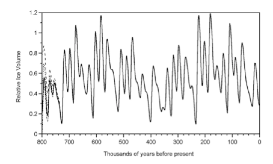
Figure 1. The LR04 benthic stack constructed by the graphic correlation of 57 globally distributed benthic δ O records (Lisieki and Raymo, 2005).
What is observed is that from about 2.7 mya to about 1.0 mya, the periodic variability of global ice volume followed a roughly 41 ky cycle, and from about 0.6 mya to the present, the global ice volume followed a much longer cycle of very roughly 90 to 110 ky. Between about 1.0 mya and 0.6 mya, a transition zone occurred in which the cycles gradually lengthened. Yet, the seemingly dominant periodic variation in summer solar input to high latitude (SIHL) due to precession was always in in force during all these eras.
Therefore, further investigation is needed to understand how the Earth system hid the effects of precession via internal dynamics. Note however, that the effects of precession were almost never completely hidden. In both the 41 ky and ~90 to 110 ky cycle regimes, smaller cyclic variations in global ice volume at a 22 ky period were superimposed on the broader cycles that had higher amplitude with longer periods. See Figure 1. Note that the benthic stack records total ice volume, not global temperature. It does record global average temperature, but only by default – and it cannot differentiate between the NH and SH (in both ice volume and temperature), which may alternate significantly.
So, one of the major challenges in understanding ice ages, is to identify why this persistent high-frequency solar signal due to the ~22 ky precessional cycle is rectified to 41 ky obliquity cycles prior to ~1.0 mya and 90 to 110 ky cycles after ~0.6 mya.
The period after about 1.0 mya is covered in the next section.
- The Last Five ice ages
The ebb and flow of northern ice sheets was driven by variations in solar input to high northern altitudes over the past ~400 ky, as shown in Figure 2. Figure 2 shows estimated temperature, but we assume this is also representative of ice volume. Each ~22 ky precession cycle exerts a higher frequency influence on growth of the ice sheets. The NH precessional maxima (up-lobes) tend to increase the northern temperature (reduce the ice volume), while the NH precessional minima tend to reduce northern temperatures (increase the ice volume). But in the period that includes the past five ice ages, there was a seemingly relentless internal drive to increase the ice sheets. Regardless of the precession cycle, the ice sheets expanded (albeit with small higher frequency overtones) until a point was reached where they disintegrated quickly.
Most solar up-lobes due to precession merely temporarily slowed down the rate of growth of the ice sheets, but did not produce a termination. Only about one out of four, or one out of five precession up-lobes produced a sudden, decisive termination. But occurrence of these terminations followed a regular pattern. While it is common to refer to this era as the “100 ky era”, closer inspection suggests that the cycles were spaced by 88 ky or 110 ky. The spacing between the 5th and 4th, and the 4th and 3rd penultimate ice ages was about 88 ky (~four precession cycles), while the spacing between the 3rd and 2nd, and the 2nd and last ice ages was about 110 ky (~five precession cycles). Evidently, the data suggest that the combination of the colder Earth, and the relentless buildup of ice and snow at high latitudes during this period resulted in the ice sheets growing faster during NH precessional minima, but retreating only somewhat during NH precessional maxima. This trend continued through four or five precession cycles, until the next precession up-lobe produced a rapid termination. It should be noted that just prior to initiation of a termination, the northern (and global) temperatures bottomed out, while CO2 dropped below 200 ppm. Ellis and Palmer (2016) provided extensive evidence that deposition of dust on the ice sheets provided a decrease in ice-albedo that acted as a trigger to enable the next precession up-lobe to melt the ice sheets. Only at the depth of an ice age (at the lowest temperature and the lowest CO2) after 4 or 5 precession cycles had evolved, would sufficient dust be deposited on the ice sheets to cause a termination. There is good evidence that Antarctic dust levels peaked prior to each termination, but we only have data for dust preceding the last termination on the northern ice sheets. And while we only have Greenland dust data for the last ice age, that data agrees well with the Antarctic dust record, so it is not unreasonable to assume that Arctic dust flux was closely correlated with Antarctic dust since the MPT.
It seems clear that the effects of higher frequency solar variations due to precession were masked by the albedo-driven tendency toward glaciation in the North, until some trigger (most likely dust) allowed a precession up-lobe to produce a termination.
The pattern during the period from 800 kya to 450 kya was not as regular as that after 450 kya, but the spacing of major glacial-interglacial periods tended to be very roughly 4 precession cycles, or at least it was more than double the 41 ky spacing of the earliest period prior to about 1 mya.
Figure 2. Comparison of mid-summer solar input to 60°N latitude to Antarctic temperature estimate over the past 800 ky.
Imbrie and Imbrie (1980) developed a simplistic model that can be written:
In which:
- y = ice volume
- x = SIHL (summer solar input to high latitude)
- T = a time constant (best fit around 17 ky)
- B = a constant to assure that ice volume builds up at a slower rate than the rate that it decays (best fit around 0.6)
This was not stated clearly in the original paper, but the variables x (SIHL) and y (ice volume) can both be positive or negative, and represent deviations from average values, rather than absolute values.
Insertion of the constant B assures that ice buildup will take place more slowly than ice sheet decay. Note that as B varies from say, 1/3 to 2/3, the ratio of effective time constants varies from 2 to 5.
Previous modelers always inserted a term y on the right side to reduce the rate of ice volume growth as the ice sheet volume increased, and increase the rate of growth as the ice volume decreased, but no physical explanations for this were offered. Inclusion of this term provides two benefits in fitting a model to the actual ice volume data:
(i) It shifts the peaks of ice volume slightly to more recent times, which helps to fit actual data.
(ii) It somewhat rectifies the higher frequencies of the SIHL (due to precession) by reducing the rate of expansion of the ice volume when the SIHL is negative, and increases the rate of expansion of the ice volume when the SIHL is positive.
Despite these factors, the application of this model to the North or to the South, nevertheless still results in a relatively “spiky” plot of ice volume vs. time. When the model is applied to the most recent 800 kyrs, the result is as shown in Figure 3 (Rapp, 2014).
Figure 3. Predicted ice volume from Imbries’ theory with T = 22,000, B = 0.6, and starting value 0.2 over the most recent 800 kyrs. (Other staring values shown as thin dashed lines lead to the same end result).
As we shall see in Section 3, this model works better in the pre-MPT period, when the ebb and flow of ice volume responded more directly to SIHL, whereas in the post-MPT period, ice volume continually built up over the years in a colder Earth, until a relatively sudden termination produced an Interglacial. In the post-MPT period, the underlying connection of SIHL to changes in ice volume is less direct and less obvious. Ellis and Palmer (2016) provided good evidence that the trigger that initiated a termination was dust deposited on the ice sheets, thus decreasing their albedo, leading to rapid melting. The Imbries’ model cannot account for this. The Imbries’ model includes the ice volume on the right side of the equation, but this is inadequate to describe events in the post-MPT era where ice continued to build up regardless of the SIHL, and only diminished when dust deposition decreased the ice albedo. In keeping with this picture of regulation of ice ages by albedo changes rather than the SIHL cycle, Best (2018) developed a model to account for this. He began with the simple equation:
dv/dt = – (1 ± b) (S)(1 – a)
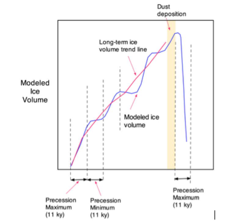
where v = ice volume, a = albedo (calculated directly from Epica dust data), S = 65°N insolation, and b is a constant inserted to make the rate of ice growth greater during precessional minima than the rate of ice loss during precessional maxima. The terms S and b require some explanation. It is assumed in this model that there is a long (88 kyr to 110 kyr) period of growth of the northern ice sheets, when the albedo remains high prior to a termination. In this long, extended period of ice sheet growth, S (measured as deviation from the average) oscillates from positive to negative due to precession, but the growth during the 11 ky precessional minima outweighs the loss during the 11 ky precessional maxima due to the high net albedo. Additionally, the plus sign is used during precessional minima, and the minus sign is used during precessional maxima. This results in alternating growth of the ice sheets through many precession cycles as shown in Figure 4 as long as the obliquity remains > 0.9.
Figure 4. Modeled alternating growth of ice sheets through precessional cycles.
At some point in time, perhaps after several precessional cycles when dust deposits have built up over the ice sheets and reduced their albedo to a critical level, the ice sheets can absorb sufficient SIHL to melt during the next precessional maximum since S > 0, and a < 0.3. In this short period (less than 11 ky) the entire termination takes place, as shown in Figure 5.
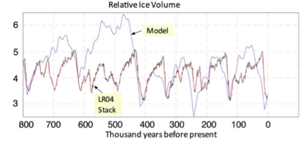
Best tried two approaches for including decreased albedo due to dust deposition in the equation based on the record of Antarctic dust in the ice cores. This assumes that Antarctic dust levels would be coupled to the dust levels on the ice sheets, but we lack data to confirm this. Best found the best fit if he assumed a 15 ky lag between the dust peak and the onset of termination. His result of integration is shown in Figure 6. While the agreement is not perfect, and could hardly be, the model captures a great deal more reality than the Imbries’ model.
Figure 5. Dust deposition precedes modeled termination.
Figure 6. Comparison of Best’s model result (blue) to LR04 stack measurement of ice volume (black) and smoother LR04 data (red).
- The Pre-MPT 41-ky Ice Age Period
It is clear from Figure 1 that during the extended period from 2.7 mya to the present:
(i) The Earth became generally colder.
(ii) The global buildup of ice and snow increased greatly during cold periods, particularly at and after 600 kya.
(iii) The spacing between cold periods increased non-linearly from 41 ky prior to the MPT to typically 4-5 precession periods after the MPT.
Raymo et al. (2006) provided a very attractive potential explanation for the 41 ky period. First of all, they emphasized that the ocean sediment data measured global ice volume, not merely northern ice volume. Secondly, they emphasized that prior to about 1.0 mya, global ice volume never reached high levels, and the high levels we associate with recent ice ages were not reached until 800 to 600 kya. A transition period (the MPT) existed between these two extremes. They then made a crucial assumption that seems very credible:
Prior to very roughly 800 kya, the buildup of ice sheets in the North was limited, and the northern ice sheets did not exert a dominant control of the global climate, as they appear to have done in the post-MPT era. In particular, the ebb and flow of Antarctic ice was controlled by the local SIHL to Antarctica, and the ebb and flow of northern ice was controlled by the local SIHL to the Arctic.
The East Antarctic Ice Sheet (EAIS) presently is ringed by extensive marine ice shelves. However, in the distant past, according to Raymo et al., “the EAIS behaved glaciologically, at that time, like a modern Greenland ice sheet… A warmer, more dynamic EAIS with a terrestrial-based melting margin, as opposed to a glacio-marine calving margin, is implied. Because such margins are strongly controlled by summer melting, Antarctic ice volume would be sensitive to orbitally driven changes in local summer insolation.”
When did the transition from terrestrial melting to calving of marine shelves take place? Until now it has been assumed that it happened between 3 and 2.6 ma. Raymo et al. proposed that it may not have happened until after 1 ma.
Based on their model, we can hypothesize that in the early period from 2.7 mya to 1.0 mya, during the 41-ky cycle era, and even extending to a rapidly diminishing degree toward 0.6 mya, that:
(i) The ice/snow in the North never built up enough in volume for its high albedo to control the global climate. Buildup and diminution of ice/snow in both the North and South merely responded to local SIHL.
(ii) In the South, ice/snow responded to SIHL much as it did in the North, as a terrestrial-based melting margin.
(iii) The global amount of ice/snow gained or lost during a complete precessional cycle is the sum of gain/loss for the North and the South. The amount of ice/snow gained in the North during the favorable half of the precession cycle is balanced by a reduction in the amount of ice/snow lost in the South. The amount of ice/snow lost in the North during the unfavorable half of the precession cycle is balanced the amount of ice/snow gained in the South. This reduces the higher frequency component due to precession in the ice volume curve, and what we are left with is simply the obliquity cycle, which enhances SIHL at both poles in synchrony.
(iv) The global total ice volume as recorded by the benthic record, is the sum of gains and losses in the North and the South, which therefore appeared to follow the obliquity signal in this era.
(v) During these smaller 41-ky ice age cycles, the total amount of global ice stored in both the North and the South, typically maximized at 50-60 m below present-day sea level and minimized at 0 to 20 m below present-day sea level. This was considerably less than maximum depression of sea level during the last five ice ages, where sea level dropped to well over 100 m below present-day sea level.
The next step is to estimate the ice volume curves in the North and South from 2.7 mya to 1.0 mya. By adding these, Raymo et al. obtained the modeled global ice volume curve.
A fundamental assumption, based on examination of the data in Figure 1, is that the rate of variation of global ice volume is proportional to solar input to high latitudes (SIHL) in the pre-MPT era. That is quite different from the post-MPT ice age era, where the relentless growth of ice sheets through 4 to 5 precession cycles was greatly modified and modulated by ice-albedo feedback influences.
Since the observed pattern of global ice volume shows a pattern with 41 kyr periodicity, and the 22 kyr periodicity only appears as relatively small perturbations superimposed on the main 41 kyr variation, the challenge is to find a mechanism for reducing the expression of the 22 kyr periodicity in the final ice volume curve.
The problem with simplistic models of how ice volume changes with SIHL is that the variation of SIHL with time is dominated by the ~22 ky precession cycles. This, in turn, causes the resultant modeled plot of ice volume vs. time to also show variability with a 22 ky period.
Raymo et al. applied the Imbries’ model to the 41 kyr period from 2.7 mya to 1.0 mya. (There is no need to include albedo in the pre-MPT period, because ice sheet extent was limited, and the effects of albedo were small. In addition, any increase in NH albedo was countered by a reduction in SH albedo, and vice versa.) Their results are shown in Figure 7. It can be seen from the lowermost graphs that the agreement of the model with experiment is surprisingly good. Inclusion of the assumed levels of SH ice volume greatly reduces the higher frequency variation due to precession, resulting in a pattern that follows only obliquity at 41 kyr cycles.
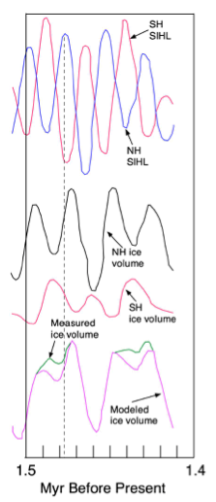
Figure 8 shows a close-up of a portion of Figure 7 from 1.5 mya to 1.4 mya, where the vertical relationship of the various curves can be followed. For example, the vertical dashed line occurs at a precession peak in NH SIHL. Reading downward along this dashed line, it can be seen that at this date, the NH ice volume is on an upward trend, but precedes the peak in NH ice volume by roughly 5,000 years. The SH SIHL is on a downward trend, but precedes the minimum in SH ice volume by roughly 8,000 years. Because the NH and SH ice volume curves are out of phase, the peaks in NH ice volume are balanced by a partial reduction in SH ice volume, and the minima in NH ice volume are balanced by a partial increase in SH ice volume, so the curve for global ice volume shows the effects of precession only as small perturbations to the underlying 41 kyr cyclic pattern.
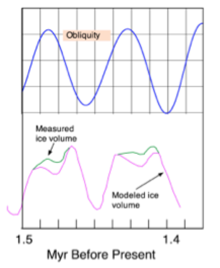
Figure 9 compares the modeled global ice volume to the obliquity. The global ice volume lags the obliquity by roughly 10 kyrs.
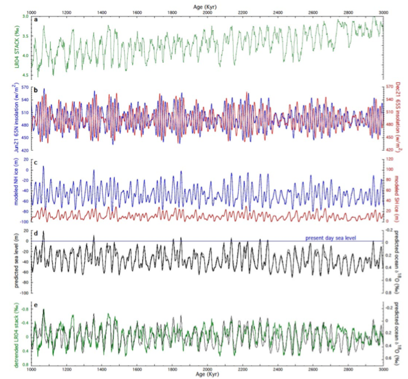
Figure 7. Age versus (A) LR04 stack of 950 benthic d18O records; (B) 65°N summer insolation records for NH (21 June) and SH (21 December); (C) NH (blue) and SH (red) modeled ice volumes; (D) predicted sea level (solid line) and mean ocean d18O (dashed line) and (E) comparison of predicted mean ocean d18O and the LR04 stack detrended by a slope of 0.8° per My from 3 to 2.5 Ma and 0.26° per My from 2.5 to 1 Ma. (Raymo et al., 2006).
Figure 8. Close-up of a portion of Figure 7.
Figure 9. Comparison of modeled ice volume to obliquity.
- Conclusions
Previous discussions suggest the following conclusions:
(1) For the whole period from 2.7 mya to the present, precession has exerted a significant higher frequency influence on the SIHL via its ~ 22 ky periodic variability.
(2) Despite the higher frequency input of precession to the SIHL, we do not observe this frequency in the record of ice volume vs. time for the whole period from 2.7 mya to the present, except as smaller secondary perturbations to underlying, more slowly varying major trends in ice volume.
(3) From about 2.7 mya to about 1.0 mya, the fundamental cadence of ice volume variability was paced by a 41 kyr period.
(4) Over the past five ice ages over the past 450 kyrs, the fundamental cadence of ice volume variability was paced by spacings of either four or five precession periods.
(5) The period from 1.0 mya to about 0.6 mya was a transition period from the 41 kyr cadence to the longer cadence, but resembled the longer cadence more closely.
(6) A major problem facing us in understanding the observations made in points 1 to 5 above, is why the higher frequency nature of the contribution of precession to the SIHL never appears in the ice volume record, except as secondary perturbations.
(7) In the earlier period from 2.7 mya to 1.0 mya, the Earth was not as cold, and buildup and decay of ice responded to local SIHL, so Arctic ice-albedo feedbacks could not dominate the Earth’s climate. During this period, the build-up and decay of Antarctic ice volume (at about 30% of northern ice volume) out of phase with northern ice volume, produced a global ice volume (sum of northern and southern) that mostly cancelled out precession variability, leaving the cycle of global ice buildup and decay appearing to only follow the 41 kyr period due to obliquity. Global ice volume never reached a level higher than about 50-60% of that in the recent ice ages.
(8) In the most recent period of the last five ice ages, and to some extent further back as far as 1.0 mya, the Earth was cold enough that the energy balance favored continued growth of the great northern ice sheets, with greater expansion during periods of low precession-induced SIHL than smaller contraction during periods of high precession-induced SIHL. The high albedo of these increasingly larger northern ice sheets could now exert a global influence on the Earth’s climate. In contrast, Antarctic ice sheets had reached their natural continental limit of expansion and so their albedo feedback remained constant, thus allowing the ever expanding NH ice sheet albedo to dominate global climate feedbacks. The ice sheets continued to grow until, after 4 or 5 precession cycles, CO2 was reduced below 200 ppm and the global temperatures reached a minimum. At that point, some factor, most likely dust accumulation on the northern ice sheets due to expansion of deserts, caused the next precessional maximum in the SIHL to relatively quickly melt the ice sheets and bring about a termination.
(9) Precession does not appear as a major factor in the history of ice volume over the past 2.7 my, even though it was always present, always active, and always important. But the final result for ice volume hid the effects of precession for totally different reasons in the early and late regimes.
References
E. Lisiecki and M. E. Raymo (2005) “A Pliocene-Pleistocene stack of 57 globally distributed benthic d18O records” Paleoceanography 20, PA1003-PA1019.
E. Raymo, L. E. Lisiecki and Kerim H. Nisancioglu (2006) “Plio-Pleistocene Ice Volume, Antarctic Climate, and the Global d18O Record” Science 313, 492-495.
Ralph Ellis, Ralph and Michael Palmer (2016) “Modulation of ice ages via precession and dust-albedo feedbacks” Geoscience Frontiers http://www.sciencedirect.com/science/article/pii/S1674987116300305
Clive Best (2018) “Towards an understanding of ice ages” http://clivebest.com/blog/?p=8679.
Donald Rapp (2014) Assessing Climate Change, 3rd ed., 816 pages, Springer, Heidelberg, ISBN-13: 978-3319004549.
John Imbrie and John Z. Imbrie (1980) “Modeling the Climatic Response to Orbital Variations” Science 207, 943-953.
Moderation note: As with all guest posts, please keep your comments civil and relevant.